In-class Exercise 4

pacman::p_load(sf, raster, spatstat, sparr, tmap, tidyverse)

geography <- st_read("data/rawdata") %>% st_union() %>% st_zm(drop = TRUE, what = "ZM") %>% st_transform(crs = 32748)

Reading layer `Kepulauan_Bangka_Belitung' from data source 
  `/home/tropicbliss/GitHub/quarto-project/In-class_Ex/In-class_Ex04/data/rawdata' 
  using driver `ESRI Shapefile'
Simple feature collection with 298 features and 27 fields
Geometry type: POLYGON
Dimension:     XYZ
Bounding box:  xmin: 105.1085 ymin: -3.116593 xmax: 106.8488 ymax: -1.501603
z_range:       zmin: 0 zmax: 0
Geodetic CRS:  WGS 84

st_as_s2(): dropping Z and/or M coordinate

Polygon Z: polygons with height data, you need to remove it.

Converting it into owin:

kbb_owin <- as.owin(geography)
kbb_owin

window: polygonal boundary
enclosing rectangle: [512066.8, 705559.4] x [9655398, 9834006] units

Checking whether it is really an owin:

class(kbb_owin)

[1] "owin"

fire_sf <- read_csv("data/rawdata/forestfires.csv") %>% st_as_sf(coords = c("longitude", "latitude"), crs = 4326) %>% st_transform(crs = 32748) # do not switch order of latlong

Rows: 741 Columns: 15
── Column specification ────────────────────────────────────────────────────────
Delimiter: ","
chr   (3): satellite, instrument, daynight
dbl  (11): latitude, longitude, brightness, scan, track, acq_time, confidenc...
date  (1): acq_date

ℹ Use `spec()` to retrieve the full column specification for this data.
ℹ Specify the column types or set `show_col_types = FALSE` to quiet this message.

Now, you want separate fields for day, month, and year for easier data filtering. The DayOfYear field takes the number of days in a year into account.

fire_sf <- fire_sf %>% mutate(DayOfYear = yday(acq_date)) %>%
  mutate(Month_num = month(acq_date)) %>%
  mutate(Month_fac = month(acq_date, label = TRUE, abbr = FALSE))

tm_shape(geography) +
  tm_polygons() +
  tm_shape(fire_sf) +
  tm_dots()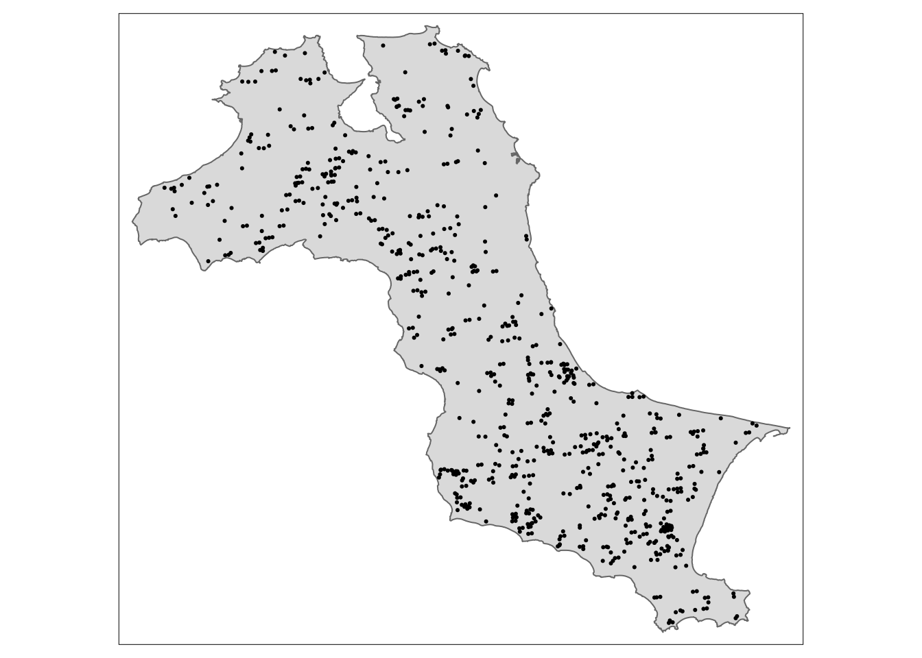

Use tm_symbols or tm_markers if you have a custom point logo.

Polygon > line > point.

A facet is a set of maps.

tm_shape(geography) +
  tm_polygons() +
  tm_shape(fire_sf) +
  tm_dots(size = 0.1) +
  tm_facets(by = "Month_fac", free.coords = FALSE, drop.units = TRUE)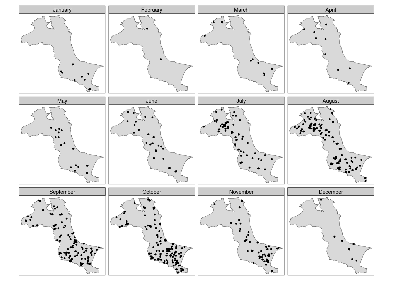

free.coords make sure that each map has the same map extent.

Extracting by month:

fire_month <- fire_sf %>% select(Month_num)

Creating ppp (to use spatstat):

fire_month_ppp <- as.ppp(fire_month)
fire_month_ppp

Marked planar point pattern: 741 points
marks are numeric, of storage type  'double'
window: rectangle = [521564.1, 695791] x [9658137, 9828767] units

summary(fire_month_ppp)

Marked planar point pattern:  741 points
Average intensity 2.49258e-08 points per square unit

Coordinates are given to 10 decimal places

marks are numeric, of type 'double'
Summary:
   Min. 1st Qu.  Median    Mean 3rd Qu.    Max. 
  1.000   8.000   9.000   8.579  10.000  12.000 

Window: rectangle = [521564.1, 695791] x [9658137, 9828767] units
                    (174200 x 170600 units)
Window area = 29728200000 square units

fire_month_owin <- fire_month_ppp[kbb_owin]
summary(fire_month_owin)

Marked planar point pattern:  741 points
Average intensity 6.424519e-08 points per square unit

Coordinates are given to 10 decimal places

marks are numeric, of type 'double'
Summary:
   Min. 1st Qu.  Median    Mean 3rd Qu.    Max. 
  1.000   8.000   9.000   8.579  10.000  12.000 

Window: polygonal boundary
2 separate polygons (no holes)
           vertices        area relative.area
polygon 1     47493 11533600000      1.00e+00
polygon 2       256      306427      2.66e-05
enclosing rectangle: [512066.8, 705559.4] x [9655398, 9834006] units
                     (193500 x 178600 units)
Window area = 11533900000 square units
Fraction of frame area: 0.334

Spatio-temporal KDE:

st_kde <- spattemp.density(fire_month_owin)

Calculating trivariate smooth...Done.
Edge-correcting...Done.
Conditioning on time...Done.

summary(st_kde)

Spatiotemporal Kernel Density Estimate

Bandwidths
  h = 15102.47 (spatial)
  lambda = 0.0304 (temporal)

No. of observations
  741 

Spatial bound
  Type: polygonal
  2D enclosure: [512066.8, 705559.4] x [9655398, 9834006]

Temporal bound
  [1, 12]

Evaluation
  128 x 128 x 12 trivariate lattice
  Density range: [1.233458e-27, 8.202976e-10]

Most of the fires started from July onwards:

tims <- c(7, 8, 9, 10, 11, 12)
par(mfcol=c(2, 3))
for (i in tims) {
  plot(st_kde, i, override.par=FALSE, fix.range=TRUE, main = paste("KDE at month", i))
}

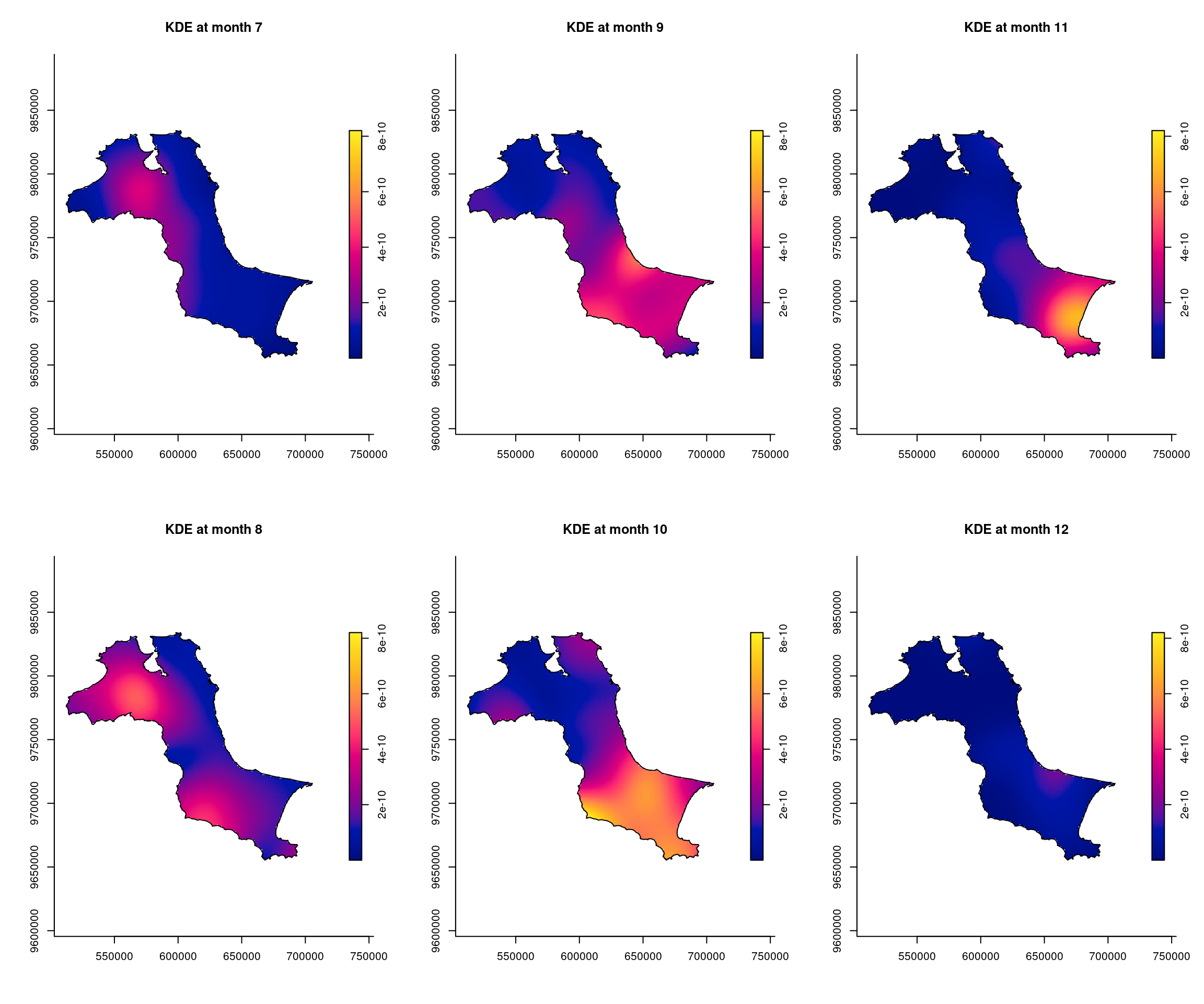
Instead of using month, you can use day which can make the value of lambda more meaningful.