pacman::p_load(sf, spdep, tmap, tidyverse)Hands-on Exercise 6
Global Measures of Spatial Autocorrelation
In this hands-on exercise, you will learn how to compute Global Measures of Spatial Autocorrelation (GMSA) by using spdep package. By the end to this hands-on exercise, you will be able to:
import geospatial data using appropriate function(s) of sf package,
import csv file using appropriate function of readr package,
perform relational join using appropriate join function of dplyr package,
compute Global Spatial Autocorrelation (GSA) statistics by using appropriate functions of spdep package,
plot Moran scatterplot,
compute and plot spatial correlogram using appropriate function of spdep package.
provide statistically correct interpretation of GSA statistics.
Since we have gone through this at the last hands-on exercise, let’s speed through this part.
Import libraries
Importing data
hunan <- st_read(dsn = "data/geospatial",
                 layer = "Hunan")
Reading layer `Hunan' from data source
`/home/tropicbliss/GitHub/quarto-project/Hands-on_Ex/Hands-on_Ex06/data/geospatial'
using driver `ESRI Shapefile'
Simple feature collection with 88 features and 7 fields
Geometry type: POLYGON
Dimension: XY
Bounding box: xmin: 108.7831 ymin: 24.6342 xmax: 114.2544 ymax: 30.12812
Geodetic CRS: WGS 84hunan2012 <- read_csv("data/aspatial/Hunan_2012.csv")Rows: 88 Columns: 29
── Column specification ────────────────────────────────────────────────────────
Delimiter: ","
chr (2): County, City
dbl (27): avg_wage, deposite, FAI, Gov_Rev, Gov_Exp, GDP, GDPPC, GIO, Loan, ...
ℹ Use `spec()` to retrieve the full column specification for this data.
ℹ Specify the column types or set `show_col_types = FALSE` to quiet this message.Data wrangling
hunan <- left_join(hunan, hunan2012) %>% select(1:4, 7, 15)Joining with `by = join_by(County)`Visualising GDPPC
equal <- tm_shape(hunan) +
  tm_fill("GDPPC",
          n = 5,
          style = "equal") +
  tm_borders(alpha = 0.5) +
  tm_layout(main.title = "Equal interval classification")

quantile <- tm_shape(hunan) +
  tm_fill("GDPPC",
          n = 5,
          style = "quantile") +
  tm_borders(alpha = 0.5) +
  tm_layout(main.title = "Equal quantile classification")

tmap_arrange(equal,
             quantile,
             asp=1,
             ncol=2)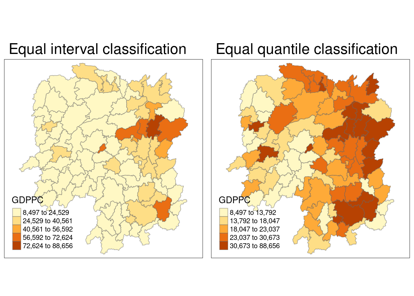
Computing contiguity spatial weights
wm_q <- poly2nb(hunan,
                queen=TRUE)
summary(wm_q)
Neighbour list object:
Number of regions: 88
Number of nonzero links: 448
Percentage nonzero weights: 5.785124
Average number of links: 5.090909
Link number distribution:
1 2 3 4 5 6 7 8 9 11
2 2 12 16 24 14 11 4 2 1
2 least connected regions:
30 65 with 1 link
1 most connected region:
85 with 11 linksRow standarised weight matrix
Next, we need to assign weights to each neighbouring polygon. Each neighboring polygon will be assigned equal weight (style=“W”) by using the fraction 1/(#ofneighbors) for each neighboring county and summing the weighted income values. While intuitive, this method can lead to over- or under-estimation along the edges of the study area due to fewer neighbors. For simplicity, we’ll use style=“W” in this example, though more robust options, such as style=“B”, are available.
rswm_q <- nb2listw(wm_q,
                   style="W",
                   zero.policy = TRUE)
rswm_q
Characteristics of weights list object:
Neighbour list object:
Number of regions: 88
Number of nonzero links: 448
Percentage nonzero weights: 5.785124
Average number of links: 5.090909
Weights style: W
Weights constants summary:
n nn S0 S1 S2
W 88 7744 88 37.86334 365.9147Moran’s I
Hypothesis testing
Now here comes the fun part. We are going to do Moran’s I testing. It measures how much nearby geographic areas are related in terms of a specific variable. It assesses whether similar or dissimilar values are clustered together in space or randomly distributed.
A positive Moran’s I indicates that similar values tend to cluster
A negative value suggests that dissimilar values are near each other
A value close to zero implies no spatial autocorrelation, meaning the values are randomly distributed across space
moran.test(hunan$GDPPC,
           listw=rswm_q,
           zero.policy = TRUE,
           na.action=na.omit)
    Moran I test under randomisation

data:  hunan$GDPPC
weights: rswm_q

Moran I statistic standard deviate = 4.7351, p-value = 1.095e-06
alternative hypothesis: greater
sample estimates:
Moran I statistic       Expectation          Variance
      0.300749970      -0.011494253       0.004348351
The Moran’s I value of 0.3007 indicates positive spatial autocorrelation in the GDP per capita (GDPPC) data, suggesting that regions with similar GDPPC values tend to cluster together.
The test’s null hypothesis assumes no spatial autocorrelation, meaning GDPPC values are randomly distributed across space.
With a p-value of 1.095e-06, which is very small, we can confidently reject the null hypothesis at conventional significance levels (e.g., 0.05 or 0.01). This provides strong statistical evidence for spatial autocorrelation in the data.
Thus, the results show a clear pattern of positive spatial autocorrelation in GDP per capita, where neighboring regions exhibit similar values.
Monte Carlo Hypothesis testing
We perform a Monte Carlo permutation test for Moran’s I to assess spatial autocorrelation in the GDPPC variable from the hunan dataset.
set.seed(1234)
bperm= moran.mc(hunan$GDPPC,
                listw=rswm_q,
                nsim=999,
                zero.policy = TRUE,
                na.action=na.omit)
bperm
    Monte-Carlo simulation of Moran I

data:  hunan$GDPPC
weights: rswm_q
number of simulations + 1: 1000

statistic = 0.30075, observed rank = 1000, p-value = 0.001
alternative hypothesis: greater
The observed Moran’s I statistic of 0.30075 indicates positive spatial autocorrelation in GDP per capita (GDPPC), meaning areas with similar GDPPC values tend to cluster.
The observed statistic ranks 1000 out of 1000 simulated values, indicating it is the largest possible, which suggests the spatial clustering is highly unusual under the assumption of no spatial autocorrelation.
With a p-value of 0.001, which is very small, we reject the null hypothesis of no spatial autocorrelation at typical significance levels (e.g., 0.05 or 0.01).
This provides strong evidence of positive spatial autocorrelation in the GDP per capita data, as the high rank and small p-value suggest the clustering is unlikely to be due to chance.
Visualisation
hist(bperm$res,
     freq=TRUE,
     breaks=20,
     xlab="Simulated Moran's I")
abline(v=0,
       col="red")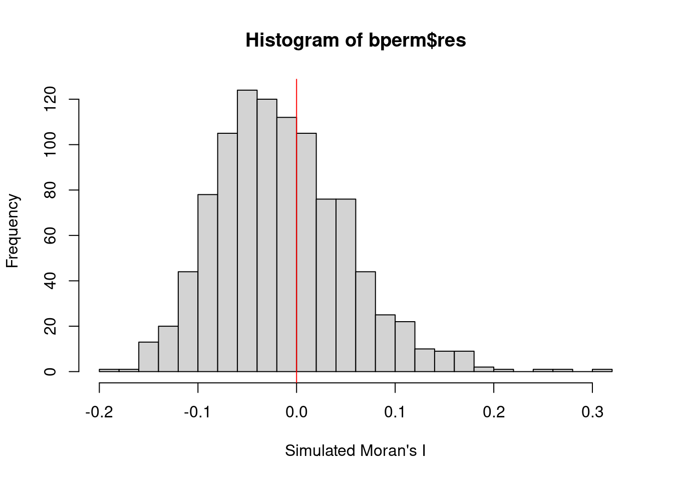
The distribution of simulated Moran’s I values with a slight rightward skew suggests that the majority of simulated Moran’s I values cluster around values less than zero or near zero. The red vertical line at 0 provides a reference for no spatial autocorrelation.
Given this rightward skew, it implies that most of the simulated values under the null hypothesis of no spatial autocorrelation tend to be lower than the observed Moran’s I statistic of 0.30075, reinforcing the conclusion that the observed Moran’s I is unusually large and indicates significant positive spatial autocorrelation in the data.
The slight rightward skew means that some of the simulated Moran’s I values are positive, but the observed Moran’s I (greater than all simulated values) is a clear outlier. This further supports the earlier conclusion that the spatial autocorrelation observed in the data is statistically significant and unlikely to be a random occurrence.
Geary’s C Test
Hypothesis testing
geary.test(hunan$GDPPC, listw=rswm_q)
    Geary C test under randomisation

data:  hunan$GDPPC
weights: rswm_q

Geary C statistic standard deviate = 3.6108, p-value = 0.0001526
alternative hypothesis: Expectation greater than statistic
sample estimates:
Geary C statistic       Expectation          Variance
        0.6907223         1.0000000         0.0073364
The observed Geary’s C statistic is 0.6907, which is below 1. Values under 1 indicate positive spatial autocorrelation, suggesting that neighboring regions in the dataset have similar GDP per capita (GDPPC) values.
The null hypothesis assumes no spatial autocorrelation, meaning GDPPC values are randomly distributed across neighboring regions.
With a p-value of 0.0001526, which is very small, we reject the null hypothesis at typical significance levels (e.g., 0.05 or 0.01), providing strong evidence of spatial autocorrelation.
The test statistic (standard deviate) of 3.6108 shows that the observed Geary’s C value significantly differs from the expected value under the null hypothesis.
This result confirms significant positive spatial autocorrelation in GDP per capita, with neighboring areas displaying similar GDPPC values, indicating local clusters of similarity.
Monte Carlo Hypothesis Testing
set.seed(1234)
bperm=geary.mc(hunan$GDPPC,
               listw=rswm_q,
               nsim=999)
bperm
    Monte-Carlo simulation of Geary C

data:  hunan$GDPPC
weights: rswm_q
number of simulations + 1: 1000

statistic = 0.69072, observed rank = 1, p-value = 0.001
alternative hypothesis: greater
The observed Geary’s C value of 0.69072, being less than 1, indicates positive spatial autocorrelation, meaning neighboring regions have similar GDP per capita (GDPPC) values.
With a rank of 1 out of 1000 simulations, the observed Geary’s C is the smallest possible value, suggesting that the spatial autocorrelation is highly unusual compared to random expectations.
The p-value of 0.001 is very small, allowing us to confidently reject the null hypothesis of no spatial autocorrelation at standard significance levels (e.g., 0.05 or 0.01).
This provides strong evidence of positive spatial autocorrelation in GDP per capita, as the low rank and small p-value confirm that the clustering of similar values is statistically significant and not due to random chance.
Visualisation
hist(bperm$res, freq=TRUE, breaks=20, xlab="Simulated Geary c")
abline(v=1, col="red") 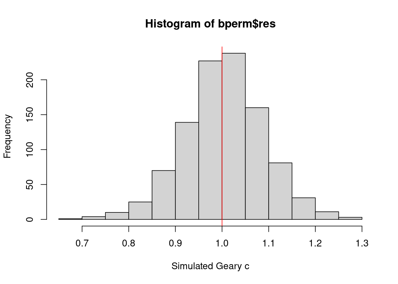
The slight leftward skew indicates that most of the simulated Geary’s C values are slightly above 1, aligning with the null hypothesis expectation of no spatial autocorrelation.
The red vertical line at 1 marks the reference point for no spatial autocorrelation. Despite the skew, while some simulated values fall below 1, most are above it. The observed Geary’s C of 0.69072, significantly lower than most simulated values, highlights the unusual and statistically significant nature of the spatial autocorrelation in the data.
In summary, the slight left skew in the histogram, along with the observed Geary’s C being well below the expected value of 1, confirms significant positive spatial autocorrelation in the dataset.
Spatial Correlogram
Spatial correlograms can help us analyse and visualize the degree of spatial autocorrelation in a dataset. Specifically, they show how the correlation between pairs of spatial observations changes as the distance (or lag) between them increases.
Moran’s I correlogram
MI_corr <- sp.correlogram(wm_q,
                          hunan$GDPPC,
                          order=6,
                          method="I",
                          style="W")
plot(MI_corr)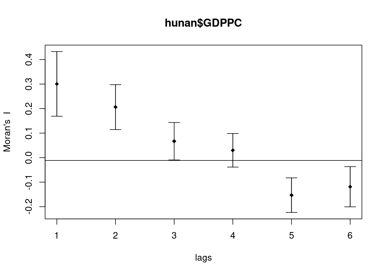
Plotting the output might not allow us to provide complete interpretation. This is because not all autocorrelation values are statistically significant. Hence, it is important for us to examine the full analysis report by printing out the analysis results as in the code chunk below.
print(MI_corr)Spatial correlogram for hunan$GDPPC
method: Moran's I
estimate expectation variance standard deviate Pr(I) two sided
1 (88) 0.3007500 -0.0114943 0.0043484 4.7351 2.189e-06 ***
2 (88) 0.2060084 -0.0114943 0.0020962 4.7505 2.029e-06 ***
3 (88) 0.0668273 -0.0114943 0.0014602 2.0496 0.040400 *
4 (88) 0.0299470 -0.0114943 0.0011717 1.2107 0.226015
5 (88) -0.1530471 -0.0114943 0.0012440 -4.0134 5.984e-05 ***
6 (88) -0.1187070 -0.0114943 0.0016791 -2.6164 0.008886 **
---
Signif. codes: 0 '***' 0.001 '**' 0.01 '*' 0.05 '.' 0.1 ' ' 1At lag 1, Moran’s I is 0.3007, indicating strong positive autocorrelation at short distances. At lag 2, Moran’s I remains positive at 0.2060, but the strength of the autocorrelation decreases as the distance increases. By lag 5, Moran’s I drops to -0.1530, indicating negative autocorrelation, meaning that dissimilar values are more likely to cluster at greater distances.
Lags 1 and 2 show highly significant positive autocorrelation, with p-values of 2.189e-06 and 2.029e-06, respectively. Lag 3 is also significant, though weaker, with a p-value of 0.0404. Lags 5 and 6 exhibit significant negative autocorrelation, with p-values of 5.984e-05 and 0.0089, respectively, while lag 4 is not significant (p-value of 0.2260).
These results suggest that hunan$GDPPC exhibits strong positive spatial autocorrelation at shorter distances (lags 1 and 2), but as distance increases, the autocorrelation weakens and becomes negative at longer distances (lags 5 and 6). This shift reflects a transition from clustering of similar values to clustering of dissimilar values as the distance between spatial units grows.
Geary’s C correlogram
GC_corr <- sp.correlogram(wm_q,
                          hunan$GDPPC,
                          order=6,
                          method="C",
                          style="W")
plot(GC_corr)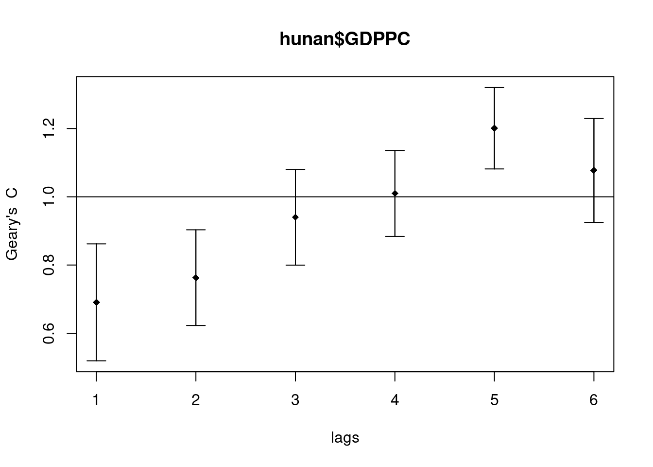
print(GC_corr)Spatial correlogram for hunan$GDPPC
method: Geary's C
estimate expectation variance standard deviate Pr(I) two sided
1 (88) 0.6907223 1.0000000 0.0073364 -3.6108 0.0003052 ***
2 (88) 0.7630197 1.0000000 0.0049126 -3.3811 0.0007220 ***
3 (88) 0.9397299 1.0000000 0.0049005 -0.8610 0.3892612
4 (88) 1.0098462 1.0000000 0.0039631 0.1564 0.8757128
5 (88) 1.2008204 1.0000000 0.0035568 3.3673 0.0007592 ***
6 (88) 1.0773386 1.0000000 0.0058042 1.0151 0.3100407
---
Signif. codes: 0 '***' 0.001 '**' 0.01 '*' 0.05 '.' 0.1 ' ' 1At lag 1, Geary’s C is 0.6907, which is below 1, indicating strong positive spatial autocorrelation. At lag 2, Geary’s C is 0.7630, still reflecting positive autocorrelation but weaker than at lag 1. By lag 5, the value of 1.2008 signals significant negative autocorrelation.
Lags 1 and 2 show highly significant positive autocorrelation, with p-values of 0.0003052 and 0.0007220, respectively. Lag 5 exhibits significant negative autocorrelation, with a p-value of 0.0007592. Lags 3, 4, and 6 do not show significant autocorrelation, as their p-values exceed 0.05.
The standard deviates show how much the observed Geary’s C diverges from the expected value of 1 under the null hypothesis of no spatial autocorrelation. Large negative standard deviates point to significant positive autocorrelation, while large positive standard deviates indicate significant negative autocorrelation.
For lags 1 and 2, strong and significant positive spatial autocorrelation is evident at shorter distances, meaning neighboring regions have similar GDP per capita. At lag 5, significant negative autocorrelation emerges, suggesting neighboring regions have dissimilar GDP values at this distance. No significant autocorrelation is detected for lags 3, 4, and 6.
This pattern reveals a shift from positive autocorrelation at shorter distances to negative autocorrelation at longer distances, reflecting a transition from clusters of similar values to clusters of dissimilar values as the distance increases.
Local Measures of Spatial Autocorrelation
Local Indicators of Spatial Association
Local Indicators of Spatial Association (LISA) are statistics used to assess the presence of clusters and/or outliers in the spatial distribution of a specific variable. For example, when analyzing the distribution of GDP per capita in Hunan Province, China, local clusters indicate that certain counties have higher or lower GDP per capita values than would be expected by random chance. In other words, the observed values are significantly higher or lower compared to what would occur in a random spatial arrangement.
Computing local Moran’s I
The localmoran() function computes Local Moran’s I statistics, which are part of the Local Indicators of Spatial Association (LISA). It identifies clusters and outliers by calculating spatial autocorrelation for individual spatial units (e.g., regions, counties) rather than the entire dataset, as global Moran’s I does.
For example, if you were analyzing the GDP per capita across different counties in a province, localmoran() would allow you to identify which counties have GDP values that are spatially autocorrelated with neighboring counties. It can highlight specific counties where GDP is either unusually high or low compared to their surroundings.
fips <- order(hunan$County)
localMI <- localmoran(hunan$GDPPC, rswm_q)
head(localMI)
Ii E.Ii Var.Ii Z.Ii Pr(z != E(Ii))
1 -0.001468468 -2.815006e-05 4.723841e-04 -0.06626904 0.9471636
2 0.025878173 -6.061953e-04 1.016664e-02 0.26266425 0.7928094
3 -0.011987646 -5.366648e-03 1.133362e-01 -0.01966705 0.9843090
4 0.001022468 -2.404783e-07 5.105969e-06 0.45259801 0.6508382
5 0.014814881 -6.829362e-05 1.449949e-03 0.39085814 0.6959021
6 -0.038793829 -3.860263e-04 6.475559e-03 -0.47728835 0.6331568printCoefmat(data.frame(
localMI[fips,],
row.names=hunan$County[fips]),
check.names=FALSE) Ii E.Ii Var.Ii Z.Ii Pr.z....E.Ii..
Anhua -2.2493e-02 -5.0048e-03 5.8235e-02 -7.2467e-02 0.9422
Anren -3.9932e-01 -7.0111e-03 7.0348e-02 -1.4791e+00 0.1391
Anxiang -1.4685e-03 -2.8150e-05 4.7238e-04 -6.6269e-02 0.9472
Baojing 3.4737e-01 -5.0089e-03 8.3636e-02 1.2185e+00 0.2230
Chaling 2.0559e-02 -9.6812e-04 2.7711e-02 1.2932e-01 0.8971
Changning -2.9868e-05 -9.0010e-09 1.5105e-07 -7.6828e-02 0.9388
Changsha 4.9022e+00 -2.1348e-01 2.3194e+00 3.3590e+00 0.0008
Chengbu 7.3725e-01 -1.0534e-02 2.2132e-01 1.5895e+00 0.1119
Chenxi 1.4544e-01 -2.8156e-03 4.7116e-02 6.8299e-01 0.4946
Cili 7.3176e-02 -1.6747e-03 4.7902e-02 3.4200e-01 0.7324
Dao 2.1420e-01 -2.0824e-03 4.4123e-02 1.0297e+00 0.3032
Dongan 1.5210e-01 -6.3485e-04 1.3471e-02 1.3159e+00 0.1882
Dongkou 5.2918e-01 -6.4461e-03 1.0748e-01 1.6338e+00 0.1023
Fenghuang 1.8013e-01 -6.2832e-03 1.3257e-01 5.1198e-01 0.6087
Guidong -5.9160e-01 -1.3086e-02 3.7003e-01 -9.5104e-01 0.3416
Guiyang 1.8240e-01 -3.6908e-03 3.2610e-02 1.0305e+00 0.3028
Guzhang 2.8466e-01 -8.5054e-03 1.4152e-01 7.7931e-01 0.4358
Hanshou 2.5878e-02 -6.0620e-04 1.0167e-02 2.6266e-01 0.7928
Hengdong 9.9964e-03 -4.9063e-04 6.7742e-03 1.2742e-01 0.8986
Hengnan 2.8064e-02 -3.2160e-04 3.7597e-03 4.6294e-01 0.6434
Hengshan -5.8201e-03 -3.0437e-05 5.1076e-04 -2.5618e-01 0.7978
Hengyang 6.2997e-02 -1.3046e-03 2.1865e-02 4.3486e-01 0.6637
Hongjiang 1.8790e-01 -2.3019e-03 3.1725e-02 1.0678e+00 0.2856
Huarong -1.5389e-02 -1.8667e-03 8.1030e-02 -4.7503e-02 0.9621
Huayuan 8.3772e-02 -8.5569e-04 2.4495e-02 5.4072e-01 0.5887
Huitong 2.5997e-01 -5.2447e-03 1.1077e-01 7.9685e-01 0.4255
Jiahe -1.2431e-01 -3.0550e-03 5.1111e-02 -5.3633e-01 0.5917
Jianghua 2.8651e-01 -3.8280e-03 8.0968e-02 1.0204e+00 0.3076
Jiangyong 2.4337e-01 -2.7082e-03 1.1746e-01 7.1800e-01 0.4728
Jingzhou 1.8270e-01 -8.5106e-04 2.4363e-02 1.1759e+00 0.2396
Jinshi -1.1988e-02 -5.3666e-03 1.1334e-01 -1.9667e-02 0.9843
Jishou -2.8680e-01 -2.6305e-03 4.4028e-02 -1.3543e+00 0.1756
Lanshan 6.3334e-02 -9.6365e-04 2.0441e-02 4.4972e-01 0.6529
Leiyang 1.1581e-02 -1.4948e-04 2.5082e-03 2.3422e-01 0.8148
Lengshuijiang -1.7903e+00 -8.2129e-02 2.1598e+00 -1.1623e+00 0.2451
Li 1.0225e-03 -2.4048e-07 5.1060e-06 4.5260e-01 0.6508
Lianyuan -1.4672e-01 -1.8983e-03 1.9145e-02 -1.0467e+00 0.2952
Liling 1.3774e+00 -1.5097e-02 4.2601e-01 2.1335e+00 0.0329
Linli 1.4815e-02 -6.8294e-05 1.4499e-03 3.9086e-01 0.6959
Linwu -2.4621e-03 -9.0703e-06 1.9258e-04 -1.7676e-01 0.8597
Linxiang 6.5904e-02 -2.9028e-03 2.5470e-01 1.3634e-01 0.8916
Liuyang 3.3688e+00 -7.7502e-02 1.5180e+00 2.7972e+00 0.0052
Longhui 8.0801e-01 -1.1377e-02 1.5538e-01 2.0787e+00 0.0376
Longshan 7.5663e-01 -1.1100e-02 3.1449e-01 1.3690e+00 0.1710
Luxi 1.8177e-01 -2.4855e-03 3.4249e-02 9.9561e-01 0.3194
Mayang 2.1852e-01 -5.8773e-03 9.8049e-02 7.1663e-01 0.4736
Miluo 1.8704e+00 -1.6927e-02 2.7925e-01 3.5715e+00 0.0004
Nan -9.5789e-03 -4.9497e-04 6.8341e-03 -1.0988e-01 0.9125
Ningxiang 1.5607e+00 -7.3878e-02 8.0012e-01 1.8274e+00 0.0676
Ningyuan 2.0910e-01 -7.0884e-03 8.2306e-02 7.5356e-01 0.4511
Pingjiang -9.8964e-01 -2.6457e-03 5.6027e-02 -4.1698e+00 0.0000
Qidong 1.1806e-01 -2.1207e-03 2.4747e-02 7.6396e-01 0.4449
Qiyang 6.1966e-02 -7.3374e-04 8.5743e-03 6.7712e-01 0.4983
Rucheng -3.6992e-01 -8.8999e-03 2.5272e-01 -7.1814e-01 0.4727
Sangzhi 2.5053e-01 -4.9470e-03 6.8000e-02 9.7972e-01 0.3272
Shaodong -3.2659e-02 -3.6592e-05 5.0546e-04 -1.4510e+00 0.1468
Shaoshan 2.1223e+00 -5.0227e-02 1.3668e+00 1.8583e+00 0.0631
Shaoyang 5.9499e-01 -1.1253e-02 1.3012e-01 1.6807e+00 0.0928
Shimen -3.8794e-02 -3.8603e-04 6.4756e-03 -4.7729e-01 0.6332
Shuangfeng 9.2835e-03 -2.2867e-03 3.1516e-02 6.5174e-02 0.9480
Shuangpai 8.0591e-02 -3.1366e-04 8.9838e-03 8.5358e-01 0.3933
Suining 3.7585e-01 -3.5933e-03 4.1870e-02 1.8544e+00 0.0637
Taojiang -2.5394e-01 -1.2395e-03 1.4477e-02 -2.1002e+00 0.0357
Taoyuan 1.4729e-02 -1.2039e-04 8.5103e-04 5.0903e-01 0.6107
Tongdao 4.6482e-01 -6.9870e-03 1.9879e-01 1.0582e+00 0.2900
Wangcheng 4.4220e+00 -1.1067e-01 1.3596e+00 3.8873e+00 0.0001
Wugang 7.1003e-01 -7.8144e-03 1.0710e-01 2.1935e+00 0.0283
Xiangtan 2.4530e-01 -3.6457e-04 3.2319e-03 4.3213e+00 0.0000
Xiangxiang 2.6271e-01 -1.2703e-03 2.1290e-02 1.8092e+00 0.0704
Xiangyin 5.4525e-01 -4.7442e-03 7.9236e-02 1.9539e+00 0.0507
Xinhua 1.1810e-01 -6.2649e-03 8.6001e-02 4.2409e-01 0.6715
Xinhuang 1.5725e-01 -4.1820e-03 3.6648e-01 2.6667e-01 0.7897
Xinning 6.8928e-01 -9.6674e-03 2.0328e-01 1.5502e+00 0.1211
Xinshao 5.7578e-02 -8.5932e-03 1.1769e-01 1.9289e-01 0.8470
Xintian -7.4050e-03 -5.1493e-03 1.0877e-01 -6.8395e-03 0.9945
Xupu 3.2406e-01 -5.7468e-03 5.7735e-02 1.3726e+00 0.1699
Yanling -6.9021e-02 -5.9211e-04 9.9306e-03 -6.8667e-01 0.4923
Yizhang -2.6844e-01 -2.2463e-03 4.7588e-02 -1.2202e+00 0.2224
Yongshun 6.3064e-01 -1.1350e-02 1.8830e-01 1.4795e+00 0.1390
Yongxing 4.3411e-01 -9.0735e-03 1.5088e-01 1.1409e+00 0.2539
You 7.8750e-02 -7.2728e-03 1.2116e-01 2.4714e-01 0.8048
Yuanjiang 2.0004e-04 -1.7760e-04 2.9798e-03 6.9181e-03 0.9945
Yuanling 8.7298e-03 -2.2981e-06 2.3221e-05 1.8121e+00 0.0700
Yueyang 4.1189e-02 -1.9768e-04 2.3113e-03 8.6085e-01 0.3893
Zhijiang 1.0476e-01 -7.8123e-04 1.3100e-02 9.2214e-01 0.3565
Zhongfang -2.2685e-01 -2.1455e-03 3.5927e-02 -1.1855e+00 0.2358
Zhuzhou 3.2864e-01 -5.2432e-04 7.2391e-03 3.8688e+00 0.0001
Zixing -7.6849e-01 -8.8210e-02 9.4057e-01 -7.0144e-01 0.4830hunan.localMI <- cbind(hunan,localMI) %>%
rename(Pr.Ii = Pr.z....E.Ii..)localMI.map <- tm_shape(hunan.localMI) +
tm_fill(col = "Ii",
style = "pretty",
title = "local moran statistics") +
tm_borders(alpha = 0.5)
pvalue.map <- tm_shape(hunan.localMI) +
tm_fill(col = "Pr.Ii",
breaks=c(-Inf, 0.001, 0.01, 0.05, 0.1, Inf),
palette="-Blues",
title = "local Moran's I p-values") +
tm_borders(alpha = 0.5)
tmap_arrange(localMI.map, pvalue.map, asp=1, ncol=2)Variable(s) "Ii" contains positive and negative values, so midpoint is set to 0. Set midpoint = NA to show the full spectrum of the color palette.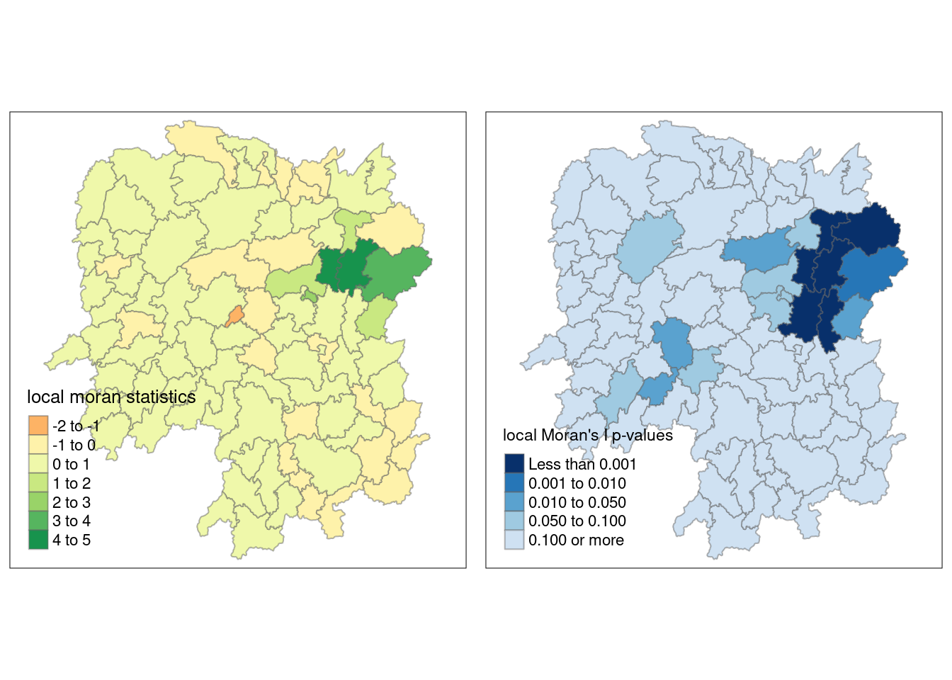
Local Moran’s I values are useful for identifying spatial clusters, showing areas where similar values (either high or low) are grouped together. A positive Local Moran’s I indicates clustering of similar values, while a negative value suggests dissimilarity between an area and its neighbors. By plotting these values, you can visualize where clusters of high or low values exist within the study area.
Local Moran’s I also detects outliers, highlighting areas with values that differ significantly from their neighbors. This can reveal places where high values are surrounded by low ones, or vice versa. Mapping these outliers helps to identify anomalies or regions that diverge from overall spatial trends.
Visualizing the p-values of Local Moran’s I helps assess the statistical significance of the spatial autocorrelation in each region. Regions with low p-values (e.g., below 0.05) are unlikely to show clustering or outliers due to random chance, adding confidence to the patterns identified.
Plotting Moran’s scatterplot
The Moran scatterplot is an illustration of the relationship between the values of the chosen attribute at each location and the average value of the same attribute at neighboring locations.
nci <- moran.plot(hunan$GDPPC, rswm_q,
                  labels=as.character(hunan$County),
                  xlab="GDPPC 2012",
                  ylab="Spatially Lag GDPPC 2012")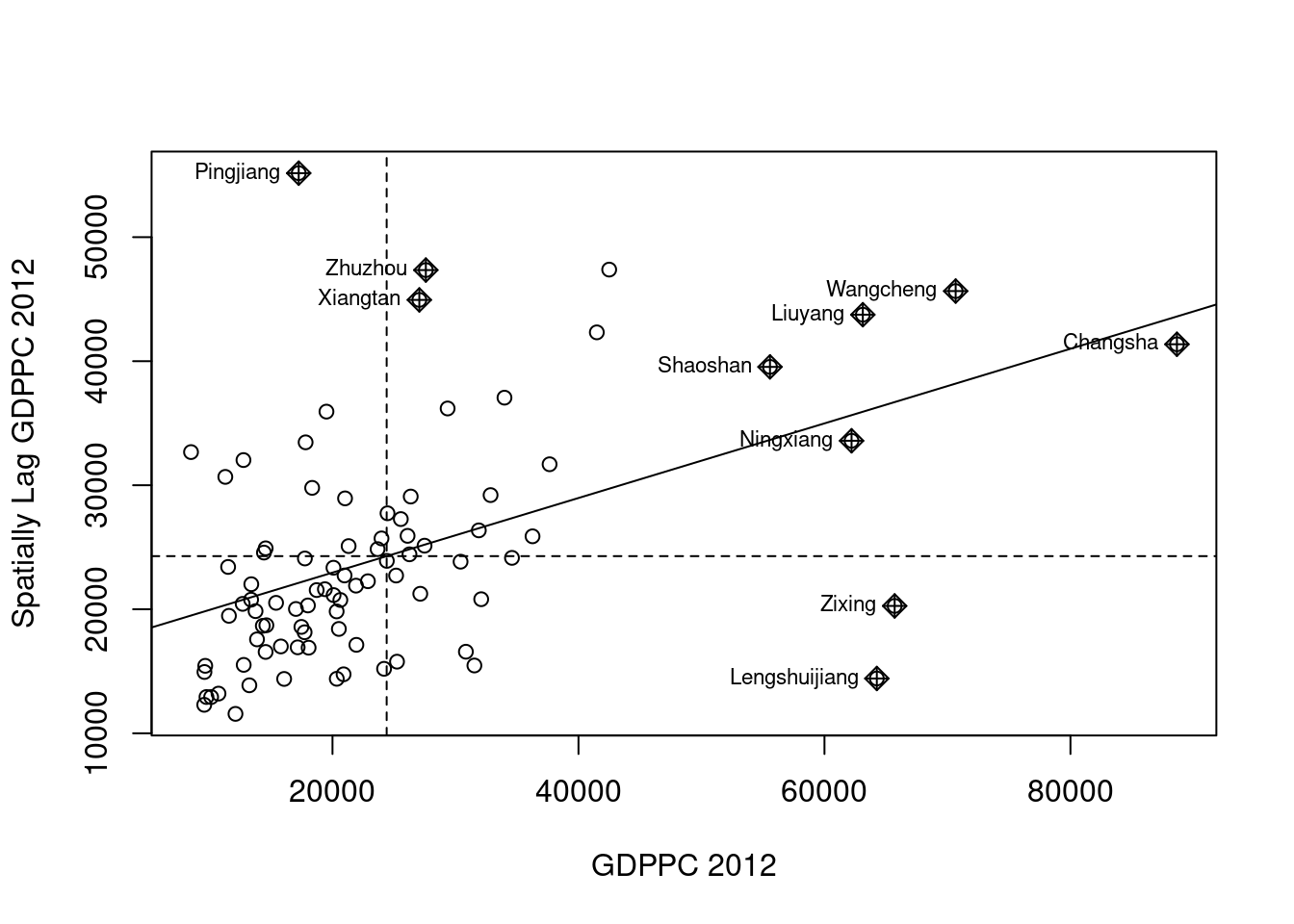
The Moran scatterplot visualizes spatial autocorrelation by depicting the relationship between a county’s GDP per capita and the average GDP per capita of its neighboring counties.
Points in the upper-right and lower-left quadrants suggest positive spatial autocorrelation, where high values are surrounded by high values or low by low. Conversely, points in the upper-left and lower-right quadrants indicate negative spatial autocorrelation, highlighting outliers where high values are surrounded by low values, or vice versa.
This plot is useful for identifying clusters of similar values (positive autocorrelation) and outliers (negative autocorrelation), with the labels helping to pinpoint the specific counties involved.
Plotting Moran’s scatterplot with standardised variable
The process of standardization involves subtracting the mean and dividing by the standard deviation, resulting in a new variable where the mean is 0 and the standard deviation is 1.
hunan$Z.GDPPC <- scale(hunan$GDPPC) %>%
  as.vector
nci2 <- moran.plot(hunan$Z.GDPPC, rswm_q,
labels=as.character(hunan$County),
xlab="z-GDPPC 2012",
ylab="Spatially Lag z-GDPPC 2012")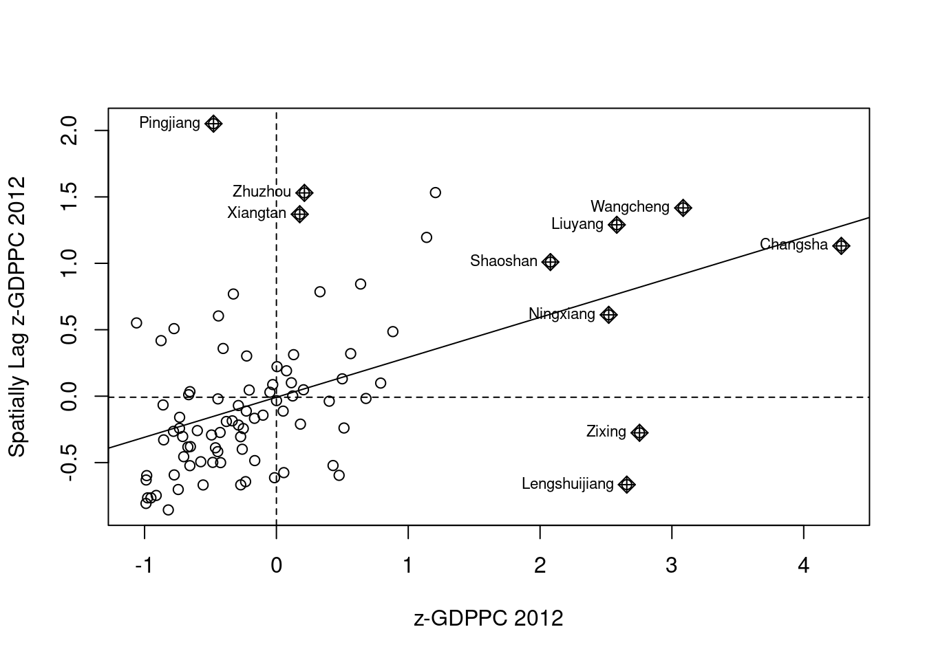
Preparing LISA map classes
This code categorizes each spatial unit into one of four quadrants according to the type of spatial autocorrelation (high-high, low-low, high-low, or low-high) determined by the local Moran’s I values and the spatial lag of GDP per capita. Units with non-significant Moran’s I values are placed in quadrant 0, signifying no significant spatial autocorrelation.
quadrant <- vector(mode="numeric",length=nrow(localMI))
hunan$lag_GDPPC <- lag.listw(rswm_q, hunan$GDPPC)
DV <- hunan$lag_GDPPC - mean(hunan$lag_GDPPC)
LM_I <- localMI[,1]
signif <- 0.05
quadrant[DV <0 & LM_I>0] <- 1
quadrant[DV >0 & LM_I<0] <- 2
quadrant[DV <0 & LM_I<0] <- 3
quadrant[DV >0 & LM_I>0] <- 4
quadrant[localMI[,5]>signif] <- 0
Plotting LISA map
hunan.localMI$quadrant <- quadrant
colors <- c("#ffffff", "#2c7bb6", "#abd9e9", "#fdae61", "#d7191c")
clusters <- c("insignificant", "low-low", "low-high", "high-low", "high-high")

tm_shape(hunan.localMI) +
  tm_fill(col = "quadrant",
          style = "cat",
          palette = colors[c(sort(unique(quadrant)))+1],
          labels = clusters[c(sort(unique(quadrant)))+1],
          popup.vars = c("")) +
  tm_view(set.zoom.limits = c(11,17)) +
  tm_borders(alpha=0.5)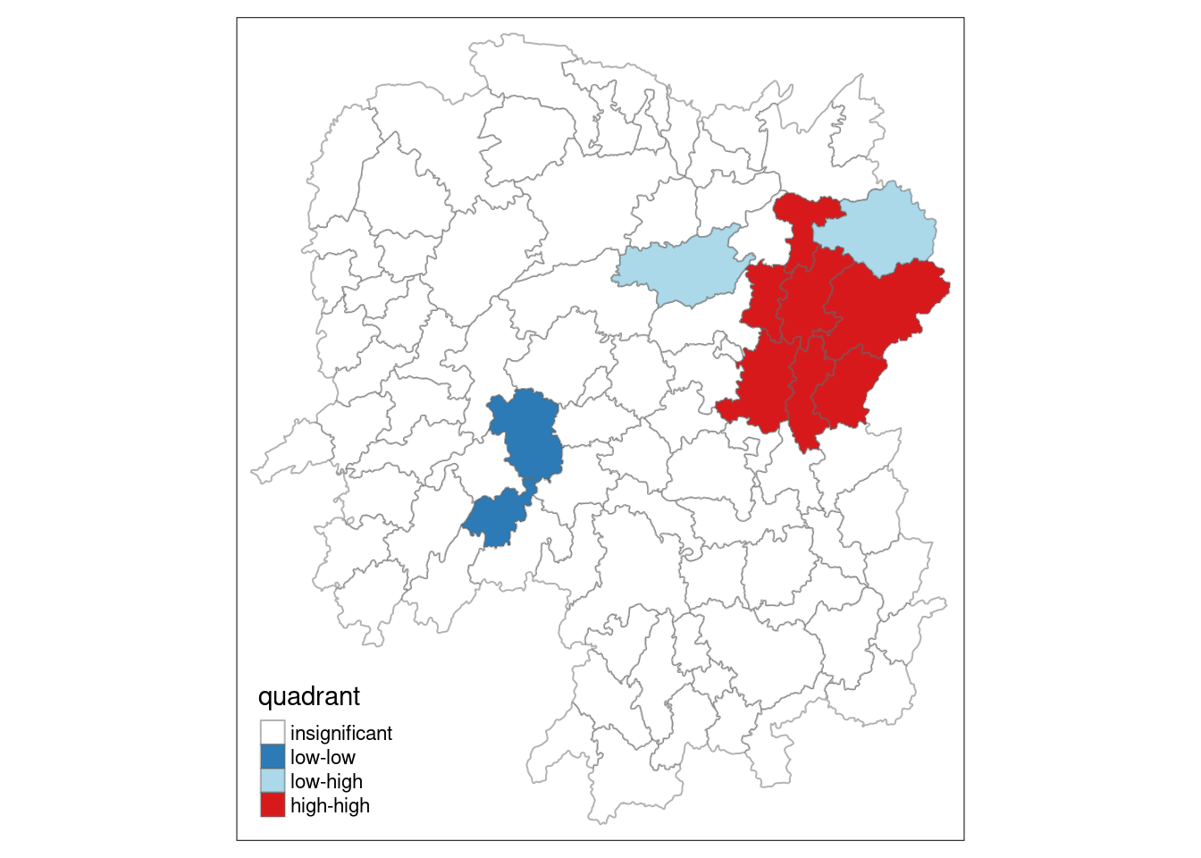
For effective interpretation, it is better to plot both the local Moran’s I values map and its corresponding p-values map next to each other.
gdppc <- qtm(hunan, "GDPPC")

hunan.localMI$quadrant <- quadrant
colors <- c("#ffffff", "#2c7bb6", "#abd9e9", "#fdae61", "#d7191c")
clusters <- c("insignificant", "low-low", "low-high", "high-low", "high-high")

LISAmap <- tm_shape(hunan.localMI) +
  tm_fill(col = "quadrant",
          style = "cat",
          palette = colors[c(sort(unique(quadrant)))+1],
          labels = clusters[c(sort(unique(quadrant)))+1],
          popup.vars = c("")) +
  tm_view(set.zoom.limits = c(11,17)) +
  tm_borders(alpha=0.5)

tmap_arrange(gdppc, LISAmap,
             asp=1, ncol=2)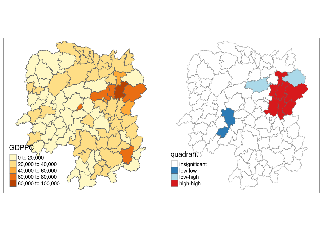
Low-high: Regions with low values and neighboring regions with high values (negative deviation with positive local Moran’s I). This quadrant identifies low-value outliers surrounded by high-value areas. For example, in the context of GDP per capita, this would indicate a county with low GDPPC surrounded by counties with high GDPPC.
High-low: Regions with high values and neighboring regions with low values (positive deviation with negative local Moran’s I). This quadrant identifies high-value outliers surrounded by low-value areas. In terms of GDP per capita, this would represent a county with high GDPPC surrounded by counties with low GDPPC.
Low-low: Regions with low values and neighboring regions also with low values (negative deviation with negative local Moran’s I). This identifies clusters of low values, where both the region and its neighbors have similarly low values. For GDPPC, this indicates a cluster of counties with low GDP per capita.
High-high: Regions with high values and neighboring regions also with high values (positive deviation with positive local Moran’s I). This identifies clusters of high values, where both the region and its neighbors have high values. In terms of GDPPC, this would represent a cluster of counties with high GDP per capita.
Hotspot and Coldspot Area Analysis
Hotspot and coldspot analysis is a spatial statistical method used to pinpoint areas where high or low values of a specific variable cluster together geographically. It aids in uncovering significant spatial patterns, emphasizing regions where extreme values, either high or low, are concentrated.
Getis and Ord’s G-statistics
We need to calculate nearest neighbours. But this time we are defining neighbours based on distance.
Deriving the centroid of each polygon
longitude <- map_dbl(hunan$geometry, ~st_centroid(.x)[[1]])
latitude <- map_dbl(hunan$geometry, ~st_centroid(.x)[[2]])
coords <- cbind(longitude, latitude)
Determining the maximum cut-off distance
k1 <- knn2nb(knearneigh(coords))Warning in knn2nb(knearneigh(coords)): neighbour object has 25 sub-graphsk1dists <- unlist(nbdists(k1, coords, longlat = TRUE))
summary(k1dists) Min. 1st Qu. Median Mean 3rd Qu. Max.
24.79 32.57 38.01 39.07 44.52 61.79 The summary report shows that the largest first nearest neighbour distance is 61.79 km, so using this as the upper threshold gives certainty that all units will have at least one neighbour.
Computing fixed distance weight matrix
wm_d62 <- dnearneigh(coords, 0, 62, longlat = TRUE)
wm_d62
Neighbour list object:
Number of regions: 88
Number of nonzero links: 324
Percentage nonzero weights: 4.183884
Average number of links: 3.681818 We then convert the nb object into a spatial weights object.
wm62_lw <- nb2listw(wm_d62, style = 'B')
summary(wm62_lw)Characteristics of weights list object:
Neighbour list object:
Number of regions: 88
Number of nonzero links: 324
Percentage nonzero weights: 4.183884
Average number of links: 3.681818
Link number distribution:
1 2 3 4 5 6
6 15 14 26 20 7
6 least connected regions:
6 15 30 32 56 65 with 1 link
7 most connected regions:
21 28 35 45 50 52 82 with 6 links
Weights style: B
Weights constants summary:
n nn S0 S1 S2
B 88 7744 324 648 5440Computing adaptive distance weight matrix
One of the characteristics of fixed distance weight matrix is that more densely settled areas (usually the urban areas) tend to have more neighbours and the less densely settled areas (usually the rural counties) tend to have lesser neighbours. Having many neighbours smoothes the neighbour relationship across more neighbours.
It is possible to control the numbers of neighbours directly using k-nearest neighbours, either accepting asymmetric neighbours or imposing symmetry as shown in the code chunk below.
knn <- knn2nb(knearneigh(coords, k=8))
knn
Neighbour list object:
Number of regions: 88
Number of nonzero links: 704
Percentage nonzero weights: 9.090909
Average number of links: 8
Non-symmetric neighbours listknn_lw <- nb2listw(knn, style = 'B')
summary(knn_lw)Characteristics of weights list object:
Neighbour list object:
Number of regions: 88
Number of nonzero links: 704
Percentage nonzero weights: 9.090909
Average number of links: 8
Non-symmetric neighbours list
Link number distribution:
8
88
88 least connected regions:
1 2 3 4 5 6 7 8 9 10 11 12 13 14 15 16 17 18 19 20 21 22 23 24 25 26 27 28 29 30 31 32 33 34 35 36 37 38 39 40 41 42 43 44 45 46 47 48 49 50 51 52 53 54 55 56 57 58 59 60 61 62 63 64 65 66 67 68 69 70 71 72 73 74 75 76 77 78 79 80 81 82 83 84 85 86 87 88 with 8 links
88 most connected regions:
1 2 3 4 5 6 7 8 9 10 11 12 13 14 15 16 17 18 19 20 21 22 23 24 25 26 27 28 29 30 31 32 33 34 35 36 37 38 39 40 41 42 43 44 45 46 47 48 49 50 51 52 53 54 55 56 57 58 59 60 61 62 63 64 65 66 67 68 69 70 71 72 73 74 75 76 77 78 79 80 81 82 83 84 85 86 87 88 with 8 links
Weights style: B
Weights constants summary:
n nn S0 S1 S2
B 88 7744 704 1300 23014Computing Gi statistics
Fixed distance
# sorts the hunan$County vector in alphabetical order and returns the indices of the sorted values
fips <- order(hunan$County)
# calculates the Getis-Ord Gi statistic* using the localG() function
# The localG() function computes the Gi* statistic for each spatial unit, returning a value that indicates whether each unit is part of a hotspot (high values) or coldspot (low values) based on the clustering of its GDP per capita values and its neighbors.
gi.fixed <- localG(hunan$GDPPC, wm62_lw)
gi.fixed
[1] 0.436075843 -0.265505650 -0.073033665 0.413017033 0.273070579
[6] -0.377510776 2.863898821 2.794350420 5.216125401 0.228236603
[11] 0.951035346 -0.536334231 0.176761556 1.195564020 -0.033020610
[16] 1.378081093 -0.585756761 -0.419680565 0.258805141 0.012056111
[21] -0.145716531 -0.027158687 -0.318615290 -0.748946051 -0.961700582
[26] -0.796851342 -1.033949773 -0.460979158 -0.885240161 -0.266671512
[31] -0.886168613 -0.855476971 -0.922143185 -1.162328599 0.735582222
[36] -0.003358489 -0.967459309 -1.259299080 -1.452256513 -1.540671121
[41] -1.395011407 -1.681505286 -1.314110709 -0.767944457 -0.192889342
[46] 2.720804542 1.809191360 -1.218469473 -0.511984469 -0.834546363
[51] -0.908179070 -1.541081516 -1.192199867 -1.075080164 -1.631075961
[56] -0.743472246 0.418842387 0.832943753 -0.710289083 -0.449718820
[61] -0.493238743 -1.083386776 0.042979051 0.008596093 0.136337469
[66] 2.203411744 2.690329952 4.453703219 -0.340842743 -0.129318589
[71] 0.737806634 -1.246912658 0.666667559 1.088613505 -0.985792573
[76] 1.233609606 -0.487196415 1.626174042 -1.060416797 0.425361422
[81] -0.837897118 -0.314565243 0.371456331 4.424392623 -0.109566928
[86] 1.364597995 -1.029658605 -0.718000620
attr(,"internals")
Gi E(Gi) V(Gi) Z(Gi) Pr(z != E(Gi))
[1,] 0.064192949 0.05747126 2.375922e-04 0.436075843 6.627817e-01
[2,] 0.042300020 0.04597701 1.917951e-04 -0.265505650 7.906200e-01
[3,] 0.044961480 0.04597701 1.933486e-04 -0.073033665 9.417793e-01
[4,] 0.039475779 0.03448276 1.461473e-04 0.413017033 6.795941e-01
[5,] 0.049767939 0.04597701 1.927263e-04 0.273070579 7.847990e-01
[6,] 0.008825335 0.01149425 4.998177e-05 -0.377510776 7.057941e-01
[7,] 0.050807266 0.02298851 9.435398e-05 2.863898821 4.184617e-03
[8,] 0.083966739 0.04597701 1.848292e-04 2.794350420 5.200409e-03
[9,] 0.115751554 0.04597701 1.789361e-04 5.216125401 1.827045e-07
[10,] 0.049115587 0.04597701 1.891013e-04 0.228236603 8.194623e-01
[11,] 0.045819180 0.03448276 1.420884e-04 0.951035346 3.415864e-01
[12,] 0.049183846 0.05747126 2.387633e-04 -0.536334231 5.917276e-01
[13,] 0.048429181 0.04597701 1.924532e-04 0.176761556 8.596957e-01
[14,] 0.034733752 0.02298851 9.651140e-05 1.195564020 2.318667e-01
[15,] 0.011262043 0.01149425 4.945294e-05 -0.033020610 9.736582e-01
[16,] 0.065131196 0.04597701 1.931870e-04 1.378081093 1.681783e-01
[17,] 0.027587075 0.03448276 1.385862e-04 -0.585756761 5.580390e-01
[18,] 0.029409313 0.03448276 1.461397e-04 -0.419680565 6.747188e-01
[19,] 0.061466754 0.05747126 2.383385e-04 0.258805141 7.957856e-01
[20,] 0.057656917 0.05747126 2.371303e-04 0.012056111 9.903808e-01
[21,] 0.066518379 0.06896552 2.820326e-04 -0.145716531 8.841452e-01
[22,] 0.045599896 0.04597701 1.928108e-04 -0.027158687 9.783332e-01
[23,] 0.030646753 0.03448276 1.449523e-04 -0.318615290 7.500183e-01
[24,] 0.035635552 0.04597701 1.906613e-04 -0.748946051 4.538897e-01
[25,] 0.032606647 0.04597701 1.932888e-04 -0.961700582 3.362000e-01
[26,] 0.035001352 0.04597701 1.897172e-04 -0.796851342 4.255374e-01
[27,] 0.012746354 0.02298851 9.812587e-05 -1.033949773 3.011596e-01
[28,] 0.061287917 0.06896552 2.773884e-04 -0.460979158 6.448136e-01
[29,] 0.014277403 0.02298851 9.683314e-05 -0.885240161 3.760271e-01
[30,] 0.009622875 0.01149425 4.924586e-05 -0.266671512 7.897221e-01
[31,] 0.014258398 0.02298851 9.705244e-05 -0.886168613 3.755267e-01
[32,] 0.005453443 0.01149425 4.986245e-05 -0.855476971 3.922871e-01
[33,] 0.043283712 0.05747126 2.367109e-04 -0.922143185 3.564539e-01
[34,] 0.020763514 0.03448276 1.393165e-04 -1.162328599 2.451020e-01
[35,] 0.081261843 0.06896552 2.794398e-04 0.735582222 4.619850e-01
[36,] 0.057419907 0.05747126 2.338437e-04 -0.003358489 9.973203e-01
[37,] 0.013497133 0.02298851 9.624821e-05 -0.967459309 3.333145e-01
[38,] 0.019289310 0.03448276 1.455643e-04 -1.259299080 2.079223e-01
[39,] 0.025996272 0.04597701 1.892938e-04 -1.452256513 1.464303e-01
[40,] 0.016092694 0.03448276 1.424776e-04 -1.540671121 1.233968e-01
[41,] 0.035952614 0.05747126 2.379439e-04 -1.395011407 1.630124e-01
[42,] 0.031690963 0.05747126 2.350604e-04 -1.681505286 9.266481e-02
[43,] 0.018750079 0.03448276 1.433314e-04 -1.314110709 1.888090e-01
[44,] 0.015449080 0.02298851 9.638666e-05 -0.767944457 4.425202e-01
[45,] 0.065760689 0.06896552 2.760533e-04 -0.192889342 8.470456e-01
[46,] 0.098966900 0.05747126 2.326002e-04 2.720804542 6.512325e-03
[47,] 0.085415780 0.05747126 2.385746e-04 1.809191360 7.042128e-02
[48,] 0.038816536 0.05747126 2.343951e-04 -1.218469473 2.230456e-01
[49,] 0.038931873 0.04597701 1.893501e-04 -0.511984469 6.086619e-01
[50,] 0.055098610 0.06896552 2.760948e-04 -0.834546363 4.039732e-01
[51,] 0.033405005 0.04597701 1.916312e-04 -0.908179070 3.637836e-01
[52,] 0.043040784 0.06896552 2.829941e-04 -1.541081516 1.232969e-01
[53,] 0.011297699 0.02298851 9.615920e-05 -1.192199867 2.331829e-01
[54,] 0.040968457 0.05747126 2.356318e-04 -1.075080164 2.823388e-01
[55,] 0.023629663 0.04597701 1.877170e-04 -1.631075961 1.028743e-01
[56,] 0.006281129 0.01149425 4.916619e-05 -0.743472246 4.571958e-01
[57,] 0.063918654 0.05747126 2.369553e-04 0.418842387 6.753313e-01
[58,] 0.070325003 0.05747126 2.381374e-04 0.832943753 4.048765e-01
[59,] 0.025947288 0.03448276 1.444058e-04 -0.710289083 4.775249e-01
[60,] 0.039752578 0.04597701 1.915656e-04 -0.449718820 6.529132e-01
[61,] 0.049934283 0.05747126 2.334965e-04 -0.493238743 6.218439e-01
[62,] 0.030964195 0.04597701 1.920248e-04 -1.083386776 2.786368e-01
[63,] 0.058129184 0.05747126 2.343319e-04 0.042979051 9.657182e-01
[64,] 0.046096514 0.04597701 1.932637e-04 0.008596093 9.931414e-01
[65,] 0.012459080 0.01149425 5.008051e-05 0.136337469 8.915545e-01
[66,] 0.091447733 0.05747126 2.377744e-04 2.203411744 2.756574e-02
[67,] 0.049575872 0.02298851 9.766513e-05 2.690329952 7.138140e-03
[68,] 0.107907212 0.04597701 1.933581e-04 4.453703219 8.440175e-06
[69,] 0.019616151 0.02298851 9.789454e-05 -0.340842743 7.332220e-01
[70,] 0.032923393 0.03448276 1.454032e-04 -0.129318589 8.971056e-01
[71,] 0.030317663 0.02298851 9.867859e-05 0.737806634 4.606320e-01
[72,] 0.019437582 0.03448276 1.455870e-04 -1.246912658 2.124295e-01
[73,] 0.055245460 0.04597701 1.932838e-04 0.666667559 5.049845e-01
[74,] 0.074278054 0.05747126 2.383538e-04 1.088613505 2.763244e-01
[75,] 0.013269580 0.02298851 9.719982e-05 -0.985792573 3.242349e-01
[76,] 0.049407829 0.03448276 1.463785e-04 1.233609606 2.173484e-01
[77,] 0.028605749 0.03448276 1.455139e-04 -0.487196415 6.261191e-01
[78,] 0.039087662 0.02298851 9.801040e-05 1.626174042 1.039126e-01
[79,] 0.031447120 0.04597701 1.877464e-04 -1.060416797 2.889550e-01
[80,] 0.064005294 0.05747126 2.359641e-04 0.425361422 6.705732e-01
[81,] 0.044606529 0.05747126 2.357330e-04 -0.837897118 4.020885e-01
[82,] 0.063700493 0.06896552 2.801427e-04 -0.314565243 7.530918e-01
[83,] 0.051142205 0.04597701 1.933560e-04 0.371456331 7.102977e-01
[84,] 0.102121112 0.04597701 1.610278e-04 4.424392623 9.671399e-06
[85,] 0.021901462 0.02298851 9.843172e-05 -0.109566928 9.127528e-01
[86,] 0.064931813 0.04597701 1.929430e-04 1.364597995 1.723794e-01
[87,] 0.031747344 0.04597701 1.909867e-04 -1.029658605 3.031703e-01
[88,] 0.015893319 0.02298851 9.765131e-05 -0.718000620 4.727569e-01
attr(,"cluster")
[1] Low Low High High High High High High High Low Low High Low Low Low
[16] High High High High Low High High Low Low High Low Low Low Low Low
[31] Low Low Low High Low Low Low Low Low Low High Low Low Low Low
[46] High High Low Low Low Low High Low Low Low Low Low High Low Low
[61] Low Low Low High High High Low High Low Low High Low High High Low
[76] High Low Low Low Low Low Low High High Low High Low Low
Levels: Low High
attr(,"gstari")
[1] FALSE
attr(,"call")
localG(x = hunan$GDPPC, listw = wm62_lw)
attr(,"class")
[1] "localG"hunan.gi <- cbind(hunan, as.matrix(gi.fixed)) %>%
rename(gstat_fixed = as.matrix.gi.fixed.)This code converts the output vector (gi.fixed) into an R matrix object using as.matrix(). Then, cbind() is applied to combine hunan@data and the gi.fixed matrix, creating a new SpatialPolygonDataFrame called hunan.gi. Finally, the field containing the gi values is renamed to gstat_fixed using rename().
gdppc <- qtm(hunan, "GDPPC")

Gimap <-tm_shape(hunan.gi) +
  tm_fill(col = "gstat_fixed",
          style = "pretty",
          palette="-RdBu",
          title = "local Gi") +
  tm_borders(alpha = 0.5)

tmap_arrange(gdppc, Gimap, asp=1, ncol=2)
Variable(s) "gstat_fixed" contains positive and negative values, so midpoint is set to 0. Set midpoint = NA to show the full spectrum of the color palette.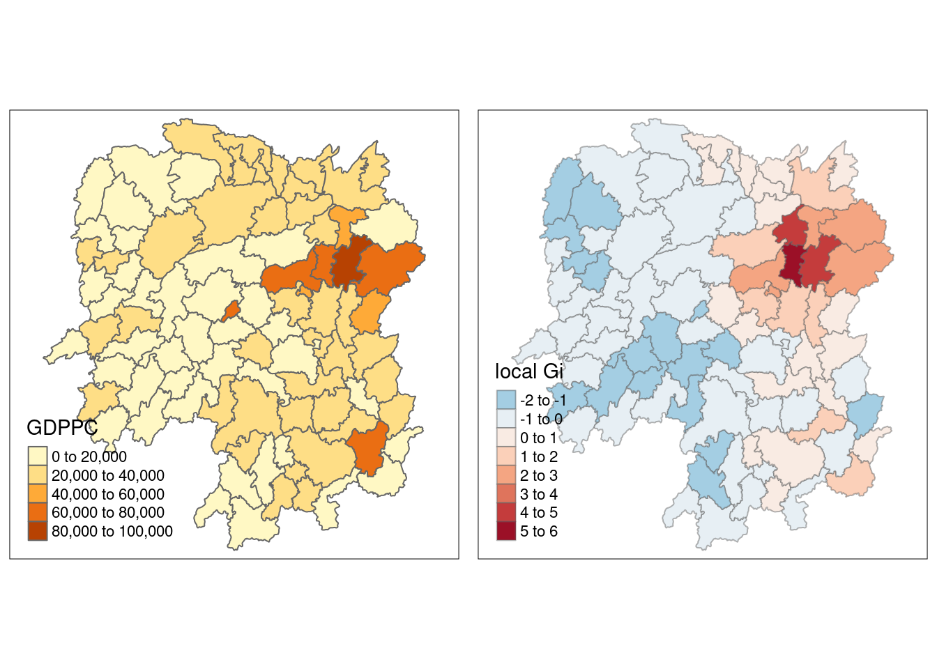
Areas with higher Gi values* in Getis-Ord Gi analysis* represent hotspots, in which regions with a higher than expected GDP per capita cluster together.
Adaptive distance
fips <- order(hunan$County)
gi.adaptive <- localG(hunan$GDPPC, knn_lw)
hunan.gi <- cbind(hunan, as.matrix(gi.adaptive)) %>%
rename(gstat_adaptive = as.matrix.gi.adaptive.)gdppc<- qtm(hunan, "GDPPC")
Gimap <- tm_shape(hunan.gi) +
tm_fill(col = "gstat_adaptive",
style = "pretty",
palette="-RdBu",
title = "local Gi") +
tm_borders(alpha = 0.5)
tmap_arrange(gdppc,
Gimap,
asp=1,
ncol=2)Variable(s) "gstat_adaptive" contains positive and negative values, so midpoint is set to 0. Set midpoint = NA to show the full spectrum of the color palette.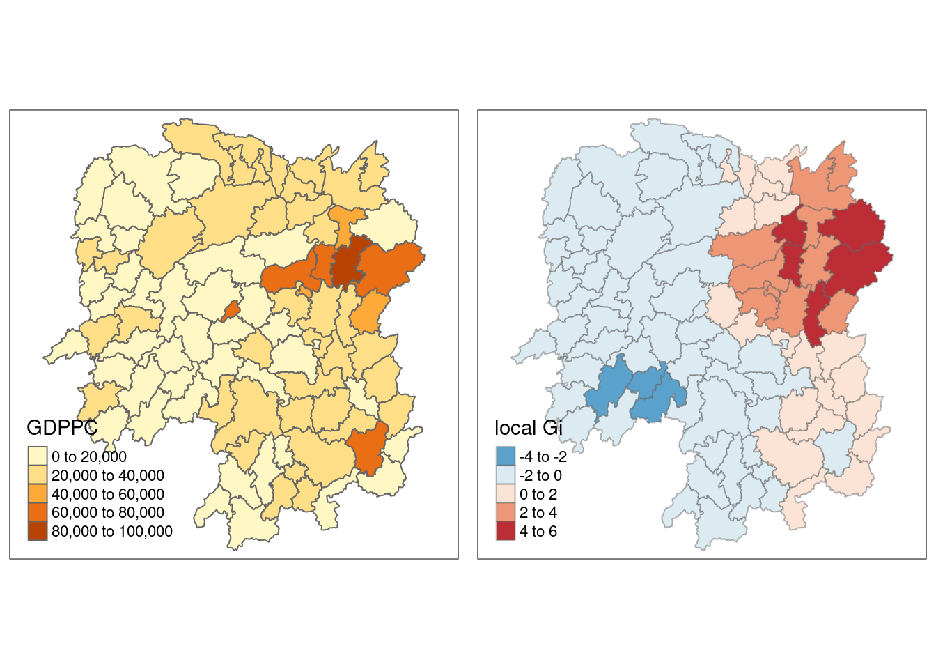
When to use fixed or adaptive distance to calculate Gi?
Fixed Distance (if all polygons are roughly the same size):
Uniform Density: Best for evenly distributed spatial units. All units are analyzed within a constant distance.
Consistent Comparisons: Ideal for comparing areas at the same scale.
Geometrically Consistent Areas: Works well for grid-like datasets.
Adaptive Distance:
Non-uniform Density: Better for unevenly distributed spatial units. Distance adjusts for each point to maintain a consistent number of neighbors.
Varying Scales: Accounts for local density variations.
Variable-Sized Neighborhoods: Ensures meaningful comparisons in both dense and sparse regions.