Hands-on Exercise 4

Author

Eugene Toh

Published

October 28, 2024

2nd Order Spatial Point Patterns Analysis Methods

Spatial Point Pattern Analysis involves assessing the distribution of points on a surface to understand underlying patterns. In this context, the points of interest are the locations of childcare centers in Singapore. The analysis seeks to answer two key questions:

  1. Are the childcare centers in Singapore randomly distributed across the country?

    • This question examines whether the placement of childcare centers follows a random pattern or if there is some underlying structure influencing their distribution.
  2. If the distribution is not random, where are the locations with a higher concentration of childcare centers?

    • This question aims to identify specific areas in Singapore that have a higher density of childcare centers, indicating potential clusters or hotspots.

Using functions from the spatstat package, the analysis will explore the spatial point processes governing the distribution of childcare centers, providing insights into the randomness or clustering of these facilities.

Importing data

pacman::p_load(sf, raster, spatstat, tmap, tidyverse)
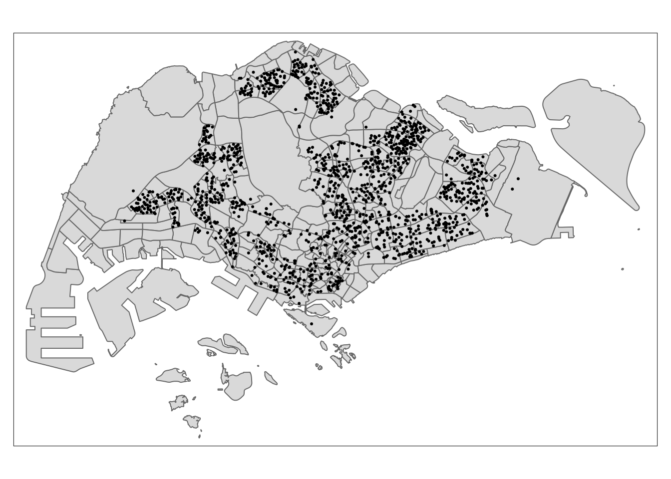
childcare_sf <- st_read("data/child-care-services-geojson.geojson") %>%
  st_transform(crs = 3414)
Reading layer `child-care-services-geojson' from data source 
  `/home/tropicbliss/GitHub/quarto-project/Hands-on_Ex/Hands-on_Ex04/data/child-care-services-geojson.geojson' 
  using driver `GeoJSON'
Simple feature collection with 1545 features and 2 fields
Geometry type: POINT
Dimension:     XYZ
Bounding box:  xmin: 103.6824 ymin: 1.248403 xmax: 103.9897 ymax: 1.462134
z_range:       zmin: 0 zmax: 0
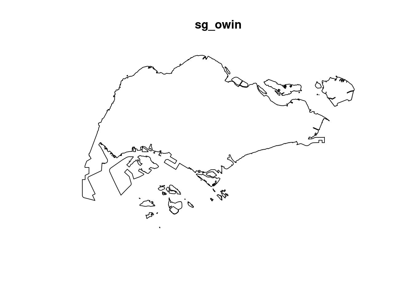
Geodetic CRS:  WGS 84
sg_sf <- st_read(dsn = "data", layer="CostalOutline")
Reading layer `CostalOutline' from data source 
  `/home/tropicbliss/GitHub/quarto-project/Hands-on_Ex/Hands-on_Ex04/data' 
  using driver `ESRI Shapefile'
Simple feature collection with 60 features and 4 fields
Geometry type: POLYGON
Dimension:     XY
Bounding box:  xmin: 2663.926 ymin: 16357.98 xmax: 56047.79 ymax: 50244.03
Projected CRS: SVY21
mpsz_sf <- st_read(dsn = "data", layer = "MP14_SUBZONE_WEB_PL")
Reading layer `MP14_SUBZONE_WEB_PL' from data source 
  `/home/tropicbliss/GitHub/quarto-project/Hands-on_Ex/Hands-on_Ex04/data' 
  using driver `ESRI Shapefile'
Simple feature collection with 323 features and 15 fields
Geometry type: MULTIPOLYGON
Dimension:     XY
Bounding box:  xmin: 2667.538 ymin: 15748.72 xmax: 56396.44 ymax: 50256.33
Projected CRS: SVY21

Now let’s check if the data imported has the correct projections:

st_crs(childcare_sf)
Coordinate Reference System:
  User input: EPSG:3414 
  wkt:
PROJCRS["SVY21 / Singapore TM",
    BASEGEOGCRS["SVY21",
        DATUM["SVY21",
            ELLIPSOID["WGS 84",6378137,298.257223563,
                LENGTHUNIT["metre",1]]],
        PRIMEM["Greenwich",0,
            ANGLEUNIT["degree",0.0174532925199433]],
        ID["EPSG",4757]],
    CONVERSION["Singapore Transverse Mercator",
        METHOD["Transverse Mercator",
            ID["EPSG",9807]],
        PARAMETER["Latitude of natural origin",1.36666666666667,
            ANGLEUNIT["degree",0.0174532925199433],
            ID["EPSG",8801]],
        PARAMETER["Longitude of natural origin",103.833333333333,
            ANGLEUNIT["degree",0.0174532925199433],
            ID["EPSG",8802]],
        PARAMETER["Scale factor at natural origin",1,
            SCALEUNIT["unity",1],
            ID["EPSG",8805]],
        PARAMETER["False easting",28001.642,
            LENGTHUNIT["metre",1],
            ID["EPSG",8806]],
        PARAMETER["False northing",38744.572,
            LENGTHUNIT["metre",1],
            ID["EPSG",8807]]],
    CS[Cartesian,2],
        AXIS["northing (N)",north,
            ORDER[1],
            LENGTHUNIT["metre",1]],
        AXIS["easting (E)",east,
            ORDER[2],
            LENGTHUNIT["metre",1]],
    USAGE[
        SCOPE["Cadastre, engineering survey, topographic mapping."],
        AREA["Singapore - onshore and offshore."],
        BBOX[1.13,103.59,1.47,104.07]],
    ID["EPSG",3414]]
st_crs(mpsz_sf)
Coordinate Reference System:
  User input: SVY21 
  wkt:
PROJCRS["SVY21",
    BASEGEOGCRS["SVY21[WGS84]",
        DATUM["World Geodetic System 1984",
            ELLIPSOID["WGS 84",6378137,298.257223563,
                LENGTHUNIT["metre",1]],
            ID["EPSG",6326]],
        PRIMEM["Greenwich",0,
            ANGLEUNIT["Degree",0.0174532925199433]]],
    CONVERSION["unnamed",
        METHOD["Transverse Mercator",
            ID["EPSG",9807]],
        PARAMETER["Latitude of natural origin",1.36666666666667,
            ANGLEUNIT["Degree",0.0174532925199433],
            ID["EPSG",8801]],
        PARAMETER["Longitude of natural origin",103.833333333333,
            ANGLEUNIT["Degree",0.0174532925199433],
            ID["EPSG",8802]],
        PARAMETER["Scale factor at natural origin",1,
            SCALEUNIT["unity",1],
            ID["EPSG",8805]],
        PARAMETER["False easting",28001.642,
            LENGTHUNIT["metre",1],
            ID["EPSG",8806]],
        PARAMETER["False northing",38744.572,
            LENGTHUNIT["metre",1],
            ID["EPSG",8807]]],
    CS[Cartesian,2],
        AXIS["(E)",east,
            ORDER[1],
            LENGTHUNIT["metre",1,
                ID["EPSG",9001]]],
        AXIS["(N)",north,
            ORDER[2],
            LENGTHUNIT["metre",1,
                ID["EPSG",9001]]]]
st_crs(sg_sf)
Coordinate Reference System:
  User input: SVY21 
  wkt:
PROJCRS["SVY21",
    BASEGEOGCRS["SVY21[WGS84]",
        DATUM["World Geodetic System 1984",
            ELLIPSOID["WGS 84",6378137,298.257223563,
                LENGTHUNIT["metre",1]],
            ID["EPSG",6326]],
        PRIMEM["Greenwich",0,
            ANGLEUNIT["Degree",0.0174532925199433]]],
    CONVERSION["unnamed",
        METHOD["Transverse Mercator",
            ID["EPSG",9807]],
        PARAMETER["Latitude of natural origin",1.36666666666667,
            ANGLEUNIT["Degree",0.0174532925199433],
            ID["EPSG",8801]],
        PARAMETER["Longitude of natural origin",103.833333333333,
            ANGLEUNIT["Degree",0.0174532925199433],
            ID["EPSG",8802]],
        PARAMETER["Scale factor at natural origin",1,
            SCALEUNIT["unity",1],
            ID["EPSG",8805]],
        PARAMETER["False easting",28001.642,
            LENGTHUNIT["metre",1],
            ID["EPSG",8806]],
        PARAMETER["False northing",38744.572,
            LENGTHUNIT["metre",1],
            ID["EPSG",8807]]],
    CS[Cartesian,2],
        AXIS["(E)",east,
            ORDER[1],
            LENGTHUNIT["metre",1,
                ID["EPSG",9001]]],
        AXIS["(N)",north,
            ORDER[2],
            LENGTHUNIT["metre",1,
                ID["EPSG",9001]]]]

Now, let’s assign the correct CRS to the following data:

mpsz_sf <- mpsz_sf %>% st_set_crs(3414)
Warning: st_crs<- : replacing crs does not reproject data; use st_transform for
that

Mapping the geospatial data sets

tmap_mode('plot')
tmap mode set to plotting
tm_shape(mpsz_sf) +
  tm_fill() + # draw polygons without borders
  tm_borders() + # draw borders
  tm_shape(childcare_sf) +
  tm_dots() # draw points

The advantage of this interactive pin map is it allows us to navigate and zoom around the map freely. We can also query the information of each simple feature (i.e. the point) by clicking of them. Last but not least, you can also change the background of the internet map layer. Currently, three internet map layers are provided. They are: ESRI.WorldGrayCanvas, OpenStreetMap, and ESRI.WorldTopoMap. The default is ESRI.WorldGrayCanvas.

Always remember to switch back to plot mode after the interactive map. This is because, each interactive mode will consume a connection. You should also avoid displaying ecessive numbers of interactive maps (i.e. not more than 10) in one RMarkdown document when publish on Netlify.

tmap_mode("plot")
tmap mode set to plotting

Now, we need to convert the generic sp objects into spatstat’s ppp object.

childcare_ppp <- as.ppp(childcare_sf)
Warning in as.ppp.sf(childcare_sf): only first attribute column is used for
marks
childcare_ppp
Marked planar point pattern: 1545 points
marks are of storage type  'character'
window: rectangle = [11203.01, 45404.24] x [25667.6, 49300.88] units

Now, let’s plot childcare_ppp:

plot(childcare_ppp)
Warning in default.charmap(ntypes, chars): Too many types to display every type
as a different character
Warning: Only 10 out of 1545 symbols are shown in the symbol map

summary(childcare_ppp)
Marked planar point pattern:  1545 points
Average intensity 1.91145e-06 points per square unit

Coordinates are given to 11 decimal places

marks are of type 'character'
Summary:
   Length     Class      Mode 
     1545 character character 

Window: rectangle = [11203.01, 45404.24] x [25667.6, 49300.88] units
                    (34200 x 23630 units)
Window area = 808287000 square units

In spatial point pattern analysis, the concept of duplicates or coincident points refers to multiple points that occupy the exact same location in space.

Many statistical methods in spatial point pattern analysis are based on the assumption that the underlying point process is simple. A simple point process means that no two points in the process can occupy the exact same location (i.e., they cannot be coincident).

If points are coincident, this assumption is violated, and the statistical methods that rely on this assumption may produce invalid or misleading results.

Thus, let’s check if there are any duplicate points:

any(duplicated(childcare_ppp))
[1] FALSE

As you can see, there doesn’t seem to be any duplicated data point.

To count the number of co-indicence point, we will use the multiplicity() function as shown in the code chunk below.

multiplicity(childcare_ppp)
   [1] 1 1 1 1 1 1 1 1 1 1 1 1 1 1 1 1 1 1 1 1 1 1 1 1 1 1 1 1 1 1 1 1 1 1 1 1 1
  [38] 1 1 1 1 1 1 1 1 1 1 1 1 1 1 1 1 1 1 1 1 1 1 1 1 1 1 1 1 1 1 1 1 1 1 1 1 1
  [75] 1 1 1 1 1 1 1 1 1 1 1 1 1 1 1 1 1 1 1 1 1 1 1 1 1 1 1 1 1 1 1 1 1 1 1 1 1
 [112] 1 1 1 1 1 1 1 1 1 1 1 1 1 1 1 1 1 1 1 1 1 1 1 1 1 1 1 1 1 1 1 1 1 1 1 1 1
 [149] 1 1 1 1 1 1 1 1 1 1 1 1 1 1 1 1 1 1 1 1 1 1 1 1 1 1 1 1 1 1 1 1 1 1 1 1 1
 [186] 1 1 1 1 1 1 1 1 1 1 1 1 1 1 1 1 1 1 1 1 1 1 1 1 1 1 1 1 1 1 1 1 1 1 1 1 1
 [223] 1 1 1 1 1 1 1 1 1 1 1 1 1 1 1 1 1 1 1 1 1 1 1 1 1 1 1 1 1 1 1 1 1 1 1 1 1
 [260] 1 1 1 1 1 1 1 1 1 1 1 1 1 1 1 1 1 1 1 1 1 1 1 1 1 1 1 1 1 1 1 1 1 1 1 1 1
 [297] 1 1 1 1 1 1 1 1 1 1 1 1 1 1 1 1 1 1 1 1 1 1 1 1 1 1 1 1 1 1 1 1 1 1 1 1 1
 [334] 1 1 1 1 1 1 1 1 1 1 1 1 1 1 1 1 1 1 1 1 1 1 1 1 1 1 1 1 1 1 1 1 1 1 1 1 1
 [371] 1 1 1 1 1 1 1 1 1 1 1 1 1 1 1 1 1 1 1 1 1 1 1 1 1 1 1 1 1 1 1 1 1 1 1 1 1
 [408] 1 1 1 1 1 1 1 1 1 1 1 1 1 1 1 1 1 1 1 1 1 1 1 1 1 1 1 1 1 1 1 1 1 1 1 1 1
 [445] 1 1 1 1 1 1 1 1 1 1 1 1 1 1 1 1 1 1 1 1 1 1 1 1 1 1 1 1 1 1 1 1 1 1 1 1 1
 [482] 1 1 1 1 1 1 1 1 1 1 1 1 1 1 1 1 1 1 1 1 1 1 1 1 1 1 1 1 1 1 1 1 1 1 1 1 1
 [519] 1 1 1 1 1 1 1 1 1 1 1 1 1 1 1 1 1 1 1 1 1 1 1 1 1 1 1 1 1 1 1 1 1 1 1 1 1
 [556] 1 1 1 1 1 1 1 1 1 1 1 1 1 1 1 1 1 1 1 1 1 1 1 1 1 1 1 1 1 1 1 1 1 1 1 1 1
 [593] 1 1 1 1 1 1 1 1 1 1 1 1 1 1 1 1 1 1 1 1 1 1 1 1 1 1 1 1 1 1 1 1 1 1 1 1 1
 [630] 1 1 1 1 1 1 1 1 1 1 1 1 1 1 1 1 1 1 1 1 1 1 1 1 1 1 1 1 1 1 1 1 1 1 1 1 1
 [667] 1 1 1 1 1 1 1 1 1 1 1 1 1 1 1 1 1 1 1 1 1 1 1 1 1 1 1 1 1 1 1 1 1 1 1 1 1
 [704] 1 1 1 1 1 1 1 1 1 1 1 1 1 1 1 1 1 1 1 1 1 1 1 1 1 1 1 1 1 1 1 1 1 1 1 1 1
 [741] 1 1 1 1 1 1 1 1 1 1 1 1 1 1 1 1 1 1 1 1 1 1 1 1 1 1 1 1 1 1 1 1 1 1 1 1 1
 [778] 1 1 1 1 1 1 1 1 1 1 1 1 1 1 1 1 1 1 1 1 1 1 1 1 1 1 1 1 1 1 1 1 1 1 1 1 1
 [815] 1 1 1 1 1 1 1 1 1 1 1 1 1 1 1 1 1 1 1 1 1 1 1 1 1 1 1 1 1 1 1 1 1 1 1 1 1
 [852] 1 1 1 1 1 1 1 1 1 1 1 1 1 1 1 1 1 1 1 1 1 1 1 1 1 1 1 1 1 1 1 1 1 1 1 1 1
 [889] 1 1 1 1 1 1 1 1 1 1 1 1 1 1 1 1 1 1 1 1 1 1 1 1 1 1 1 1 1 1 1 1 1 1 1 1 1
 [926] 1 1 1 1 1 1 1 1 1 1 1 1 1 1 1 1 1 1 1 1 1 1 1 1 1 1 1 1 1 1 1 1 1 1 1 1 1
 [963] 1 1 1 1 1 1 1 1 1 1 1 1 1 1 1 1 1 1 1 1 1 1 1 1 1 1 1 1 1 1 1 1 1 1 1 1 1
[1000] 1 1 1 1 1 1 1 1 1 1 1 1 1 1 1 1 1 1 1 1 1 1 1 1 1 1 1 1 1 1 1 1 1 1 1 1 1
[1037] 1 1 1 1 1 1 1 1 1 1 1 1 1 1 1 1 1 1 1 1 1 1 1 1 1 1 1 1 1 1 1 1 1 1 1 1 1
[1074] 1 1 1 1 1 1 1 1 1 1 1 1 1 1 1 1 1 1 1 1 1 1 1 1 1 1 1 1 1 1 1 1 1 1 1 1 1
[1111] 1 1 1 1 1 1 1 1 1 1 1 1 1 1 1 1 1 1 1 1 1 1 1 1 1 1 1 1 1 1 1 1 1 1 1 1 1
[1148] 1 1 1 1 1 1 1 1 1 1 1 1 1 1 1 1 1 1 1 1 1 1 1 1 1 1 1 1 1 1 1 1 1 1 1 1 1
[1185] 1 1 1 1 1 1 1 1 1 1 1 1 1 1 1 1 1 1 1 1 1 1 1 1 1 1 1 1 1 1 1 1 1 1 1 1 1
[1222] 1 1 1 1 1 1 1 1 1 1 1 1 1 1 1 1 1 1 1 1 1 1 1 1 1 1 1 1 1 1 1 1 1 1 1 1 1
[1259] 1 1 1 1 1 1 1 1 1 1 1 1 1 1 1 1 1 1 1 1 1 1 1 1 1 1 1 1 1 1 1 1 1 1 1 1 1
[1296] 1 1 1 1 1 1 1 1 1 1 1 1 1 1 1 1 1 1 1 1 1 1 1 1 1 1 1 1 1 1 1 1 1 1 1 1 1
[1333] 1 1 1 1 1 1 1 1 1 1 1 1 1 1 1 1 1 1 1 1 1 1 1 1 1 1 1 1 1 1 1 1 1 1 1 1 1
[1370] 1 1 1 1 1 1 1 1 1 1 1 1 1 1 1 1 1 1 1 1 1 1 1 1 1 1 1 1 1 1 1 1 1 1 1 1 1
[1407] 1 1 1 1 1 1 1 1 1 1 1 1 1 1 1 1 1 1 1 1 1 1 1 1 1 1 1 1 1 1 1 1 1 1 1 1 1
[1444] 1 1 1 1 1 1 1 1 1 1 1 1 1 1 1 1 1 1 1 1 1 1 1 1 1 1 1 1 1 1 1 1 1 1 1 1 1
[1481] 1 1 1 1 1 1 1 1 1 1 1 1 1 1 1 1 1 1 1 1 1 1 1 1 1 1 1 1 1 1 1 1 1 1 1 1 1
[1518] 1 1 1 1 1 1 1 1 1 1 1 1 1 1 1 1 1 1 1 1 1 1 1 1 1 1 1 1

If we want to know how many locations have more than one point event, we can use the code chunk below:

sum(multiplicity(childcare_ppp) > 1)
[1] 0

To view the locations of any duplicate point events, we will plot childcare data by using the code chunk below:

coincident_points <- childcare_sf[duplicated(st_geometry(childcare_sf)), ]
tmap_mode('view')
tmap mode set to interactive viewing
tm_shape(coincident_points) +
  tm_dots(alpha=0.4, 
          size=0.05)
tmap_mode("plot")
tmap mode set to plotting

There are three ways to overcome this problem. The easiest way is to delete the duplicates. But, that will also mean that some useful point events will be lost.

The second solution is use jittering. It is used to add a small amount of random noise to the coordinates of points in a spatial point pattern. This process, often referred to as “jittering,” helps to separate coincident points (points that have the exact same coordinates) by moving them slightly apart. This can be particularly useful in spatial analyses where coincident points might violate assumptions, such as the assumption that points are not exactly coincident.

The third solution is to make each point “unique” and then attach the duplicates of the points to the patterns as marks, as attributes of the points. Then you would need analytical techniques that take into account these marks.

The code chunk below implements the jittering approach.

childcare_ppp_jit <- rjitter(childcare_ppp, 
                             retry=TRUE, 
                             nsim=1, 
                             drop=TRUE)

Let’s see if there are any duplicates now:

any(duplicated(childcare_ppp_jit))
[1] FALSE

Creating owin object

When analysing spatial point patterns, it is a good practice to confine the analysis with a geographical area like Singapore boundary. In spatstat, an object called owin is specially designed to represent this polygonal region.

The code chunk below is used to covert sg SpatialPolygon object into owin object of spatstat.

sg_owin <- as.owin(sg_sf)

The ouput object can be displayed by using plot() function

plot(sg_owin)

summary(sg_owin)
Window: polygonal boundary
50 separate polygons (1 hole)
                 vertices         area relative.area
polygon 1 (hole)       30     -7081.18     -9.76e-06
polygon 2              55     82537.90      1.14e-04
polygon 3              90    415092.00      5.72e-04
polygon 4              49     16698.60      2.30e-05
polygon 5              38     24249.20      3.34e-05
polygon 6             976  23344700.00      3.22e-02
polygon 7             721   1927950.00      2.66e-03
polygon 8            1992   9992170.00      1.38e-02
polygon 9             330   1118960.00      1.54e-03
polygon 10            175    925904.00      1.28e-03
polygon 11            115    928394.00      1.28e-03
polygon 12             24      6352.39      8.76e-06
polygon 13            190    202489.00      2.79e-04
polygon 14             37     10170.50      1.40e-05
polygon 15             25     16622.70      2.29e-05
polygon 16             10      2145.07      2.96e-06
polygon 17             66     16184.10      2.23e-05
polygon 18           5195 636837000.00      8.78e-01
polygon 19             76    312332.00      4.31e-04
polygon 20            627  31891300.00      4.40e-02
polygon 21             20     32842.00      4.53e-05
polygon 22             42     55831.70      7.70e-05
polygon 23             67   1313540.00      1.81e-03
polygon 24            734   4690930.00      6.47e-03
polygon 25             16      3194.60      4.40e-06
polygon 26             15      4872.96      6.72e-06
polygon 27             15      4464.20      6.15e-06
polygon 28             14      5466.74      7.54e-06
polygon 29             37      5261.94      7.25e-06
polygon 30            111    662927.00      9.14e-04
polygon 31             69     56313.40      7.76e-05
polygon 32            143    145139.00      2.00e-04
polygon 33            397   2488210.00      3.43e-03
polygon 34             90    115991.00      1.60e-04
polygon 35             98     62682.90      8.64e-05
polygon 36            165    338736.00      4.67e-04
polygon 37            130     94046.50      1.30e-04
polygon 38             93    430642.00      5.94e-04
polygon 39             16      2010.46      2.77e-06
polygon 40            415   3253840.00      4.49e-03
polygon 41             30     10838.20      1.49e-05
polygon 42             53     34400.30      4.74e-05
polygon 43             26      8347.58      1.15e-05
polygon 44             74     58223.40      8.03e-05
polygon 45            327   2169210.00      2.99e-03
polygon 46            177    467446.00      6.44e-04
polygon 47             46    699702.00      9.65e-04
polygon 48              6     16841.00      2.32e-05
polygon 49             13     70087.30      9.66e-05
polygon 50              4      9459.63      1.30e-05
enclosing rectangle: [2663.93, 56047.79] x [16357.98, 50244.03] units
                     (53380 x 33890 units)
Window area = 725376000 square units
Fraction of frame area: 0.401

Combining point events object and owin object

In this last step of geospatial data wrangling, we will extract childcare events that are located within Singapore by using the code chunk below.

childcareSG_ppp = childcare_ppp[sg_owin]
summary(childcareSG_ppp)
Marked planar point pattern:  1545 points
Average intensity 2.129929e-06 points per square unit

Coordinates are given to 11 decimal places

marks are of type 'character'
Summary:
   Length     Class      Mode 
     1545 character character 

Window: polygonal boundary
50 separate polygons (1 hole)
                 vertices         area relative.area
polygon 1 (hole)       30     -7081.18     -9.76e-06
polygon 2              55     82537.90      1.14e-04
polygon 3              90    415092.00      5.72e-04
polygon 4              49     16698.60      2.30e-05
polygon 5              38     24249.20      3.34e-05
polygon 6             976  23344700.00      3.22e-02
polygon 7             721   1927950.00      2.66e-03
polygon 8            1992   9992170.00      1.38e-02
polygon 9             330   1118960.00      1.54e-03
polygon 10            175    925904.00      1.28e-03
polygon 11            115    928394.00      1.28e-03
polygon 12             24      6352.39      8.76e-06
polygon 13            190    202489.00      2.79e-04
polygon 14             37     10170.50      1.40e-05
polygon 15             25     16622.70      2.29e-05
polygon 16             10      2145.07      2.96e-06
polygon 17             66     16184.10      2.23e-05
polygon 18           5195 636837000.00      8.78e-01
polygon 19             76    312332.00      4.31e-04
polygon 20            627  31891300.00      4.40e-02
polygon 21             20     32842.00      4.53e-05
polygon 22             42     55831.70      7.70e-05
polygon 23             67   1313540.00      1.81e-03
polygon 24            734   4690930.00      6.47e-03
polygon 25             16      3194.60      4.40e-06
polygon 26             15      4872.96      6.72e-06
polygon 27             15      4464.20      6.15e-06
polygon 28             14      5466.74      7.54e-06
polygon 29             37      5261.94      7.25e-06
polygon 30            111    662927.00      9.14e-04
polygon 31             69     56313.40      7.76e-05
polygon 32            143    145139.00      2.00e-04
polygon 33            397   2488210.00      3.43e-03
polygon 34             90    115991.00      1.60e-04
polygon 35             98     62682.90      8.64e-05
polygon 36            165    338736.00      4.67e-04
polygon 37            130     94046.50      1.30e-04
polygon 38             93    430642.00      5.94e-04
polygon 39             16      2010.46      2.77e-06
polygon 40            415   3253840.00      4.49e-03
polygon 41             30     10838.20      1.49e-05
polygon 42             53     34400.30      4.74e-05
polygon 43             26      8347.58      1.15e-05
polygon 44             74     58223.40      8.03e-05
polygon 45            327   2169210.00      2.99e-03
polygon 46            177    467446.00      6.44e-04
polygon 47             46    699702.00      9.65e-04
polygon 48              6     16841.00      2.32e-05
polygon 49             13     70087.30      9.66e-05
polygon 50              4      9459.63      1.30e-05
enclosing rectangle: [2663.93, 56047.79] x [16357.98, 50244.03] units
                     (53380 x 33890 units)
Window area = 725376000 square units
Fraction of frame area: 0.401
plot(childcareSG_ppp)
Warning in default.charmap(ntypes, chars): Too many types to display every type
as a different character
Warning: Only 10 out of 1545 symbols are shown in the symbol map

Comparing Spatial Point Patterns using KDE

In this section, you will learn how to compare KDE of childcare at Ponggol, Tampines, Chua Chu Kang and Jurong West planning areas.

The code chunk below will be used to extract the target planning areas.

pg <- mpsz_sf %>%
  filter(PLN_AREA_N == "PUNGGOL")
tm <- mpsz_sf %>%
  filter(PLN_AREA_N == "TAMPINES")
ck <- mpsz_sf %>%
  filter(PLN_AREA_N == "CHOA CHU KANG")
jw <- mpsz_sf %>%
  filter(PLN_AREA_N == "JURONG WEST")

Plotting target planning areas:

par(mfrow=c(2,2))
plot(pg, main = "Ponggol")
Warning: plotting the first 9 out of 15 attributes; use max.plot = 15 to plot
all

plot(tm, main = "Tampines")
Warning: plotting the first 9 out of 15 attributes; use max.plot = 15 to plot
all

plot(ck, main = "Choa Chu Kang")
Warning: plotting the first 10 out of 15 attributes; use max.plot = 15 to plot
all

plot(jw, main = "Jurong West")
Warning: plotting the first 9 out of 15 attributes; use max.plot = 15 to plot
all

Now, we will convert these sf objects into owin objects that is required by spatstat.

pg_owin = as.owin(pg)
tm_owin = as.owin(tm)
ck_owin = as.owin(ck)
jw_owin = as.owin(jw)

By using the code chunk below, we are able to extract childcare that is within the specific region to do our analysis later on.

Now why would you bother to split them up? To analyse spatial randomness it is essential to exclude regions like the airport where there are no childcare centres.

childcare_pg_ppp = childcare_ppp_jit[pg_owin]
childcare_tm_ppp = childcare_ppp_jit[tm_owin]
childcare_ck_ppp = childcare_ppp_jit[ck_owin]
childcare_jw_ppp = childcare_ppp_jit[jw_owin]

Next, rescale.ppp() function is used to trasnform the unit of measurement from metre to kilometre.

childcare_pg_ppp.km = rescale.ppp(childcare_pg_ppp, 1000, "km")
childcare_tm_ppp.km = rescale.ppp(childcare_tm_ppp, 1000, "km")
childcare_ck_ppp.km = rescale.ppp(childcare_ck_ppp, 1000, "km")
childcare_jw_ppp.km = rescale.ppp(childcare_jw_ppp, 1000, "km")

The code chunk below is used to plot these four study areas and the locations of the childcare centres.

par(mfrow=c(2,2))
plot(childcare_pg_ppp.km, main="Punggol")
Warning in default.charmap(ntypes, chars): Too many types to display every type
as a different character
Warning: Only 10 out of 61 symbols are shown in the symbol map
plot(childcare_tm_ppp.km, main="Tampines")
Warning in default.charmap(ntypes, chars): Too many types to display every type
as a different character
Warning: Only 10 out of 89 symbols are shown in the symbol map
plot(childcare_ck_ppp.km, main="Choa Chu Kang")
Warning in default.charmap(ntypes, chars): Too many types to display every type
as a different character
Warning: Only 10 out of 61 symbols are shown in the symbol map
plot(childcare_jw_ppp.km, main="Jurong West")
Warning in default.charmap(ntypes, chars): Too many types to display every type
as a different character
Warning: Only 10 out of 88 symbols are shown in the symbol map

Analysing Spatial Point Process Using G-Function

The G function measures the distribution of the distances from an arbitrary event to its nearest event. In this section, you will learn how to compute G-function estimation by using Gest() of spatstat package. You will also learn how to perform monta carlo simulation test using envelope() of spatstat package.

Note that it is typical for randomness to occur when the area of analysis is high. It is important to figure out that at what distance does clustering occur and at what distance randomness starts to appear again. This can be done using the L function. We can further modify the L function to make it from a diagonal to a straight line. We have lots of different functions, like G function (zonal - within a ring buffer, how many points are there, and slowly draw more and more bigger rings, so unlike K function it is not cumulative, there is no straight version of it) or K function (the L function is the same as the K function except a transformation is applied to the result to make the graph straight, making it easier to interpret). Each employ a different shape but they are all distance based. Some analyse distances zone by zone while some are cumulative.

It essentially answers the question: “given a point in the spatial pattern, what is the probability that the nearest neighboring point is within a certain distance r”?

  • x-axis (r): This represents the distance (in the same units as your spatial data).

  • y-axis (G(r)): This is the cumulative probability that the nearest neighbor distance is less than or equal to r.

Computing G-function estimation

The code chunk below is used to compute G-function using Gest() of spatat package for the Chua Chu Kang planning area.

G_CK = Gest(childcare_ck_ppp, correction = "border")
plot(G_CK, xlim=c(0,500))

If the curve rises steeply at short distances, it indicates that most points have a nearby neighbor, suggesting a clustered pattern. If the curve rises more gradually, it indicates a more dispersed pattern where points are further apart on average. A linear increase in the G-function typically suggests a random or Poisson process, where points are randomly distributed. If you have plotted the theoretical G-function (usually a straight line), deviations from this line indicate either clustering (curve above the theoretical line) or regularity (curve below the theoretical line).

The correction = "border" parameter adjusts the G-function to account for edge effects, which occur because points near the boundary of the study region have fewer neighboring points within the study area.

xlim=c(0,500) limits the distance axis to between 0 and 500 units. You would analyze the curve within this range to understand the distribution of nearest neighbor distances among your spatial points.

Now for the Tampines planning area:

G_tm = Gest(childcare_tm_ppp, correction = "best")
plot(G_tm)

Hypothesis testing

To confirm the observed spatial patterns above, a hypothesis test will be conducted. The hypothesis and test are as follows:

Ho = The distribution of childcare services at Choa Chu Kang are randomly distributed.

H1= The distribution of childcare services at Choa Chu Kang are not randomly distributed.

The null hypothesis will be rejected if p-value is smaller than alpha value of 0.001.

G_CK.csr <- envelope(childcare_ck_ppp, Gest, nsim = 999)
Generating 999 simulations of CSR  ...
1, 2, 3, ......10.........20.........30.........40.........50.........60..
.......70.........80.........90.........100.........110.........120.........130
.........140.........150.........160.........170.........180.........190........
.200.........210.........220.........230.........240.........250.........260......
...270.........280.........290.........300.........310.........320.........330....
.....340.........350.........360.........370.........380.........390.........400..
.......410.........420.........430.........440.........450.........460.........470
.........480.........490.........500.........510.........520.........530........
.540.........550.........560.........570.........580.........590.........600......
...610.........620.........630.........640.........650.........660.........670....
.....680.........690.........700.........710.........720.........730.........740..
.......750.........760.........770.........780.........790.........800.........810
.........820.........830.........840.........850.........860.........870........
.880.........890.........900.........910.........920.........930.........940......
...950.........960.........970.........980.........990........
999.

Done.

Since you are using more simulation iterations, the time taken to run the tests will be longer. Since this is essentially Monte Carlo simulation, to satisfy a 95% confidence interval, we need a minimum of 39 for convergence. 99, 199, 999 are common values. We need a greater amount to achieve a more stable result. Note that 99 means that you are running it 100 times.

plot(G_CK.csr)

For the Tampines planning area:

G_tm.csr <- envelope(childcare_tm_ppp, Gest, correction = "all", nsim = 999)
Generating 999 simulations of CSR  ...
1, 2, 3, ......10.........20.........30.........40.........50.........60..
.......70.........80.........90.........100.........110.........120.........130
.........140.........150.........160.........170.........180.........190........
.200.........210.........220.........230.........240.........250.........260......
...270.........280.........290.........300.........310.........320.........330....
.....340.........350.........360.........370.........380.........390.........400..
.......410.........420.........430.........440.........450.........460.........470
.........480.........490.........500.........510.........520.........530........
.540.........550.........560.........570.........580.........590.........600......
...610.........620.........630.........640.........650.........660.........670....
.....680.........690.........700.........710.........720.........730.........740..
.......750.........760.........770.........780.........790.........800.........810
.........820.........830.........840.........850.........860.........870........
.880.........890.........900.........910.........920.........930.........940......
...950.........960.........970.........980.........990........
999.

Done.
plot(G_tm.csr)

Note that it is typical for randomness to occur when the area of analysis is high. It is important to figure out that at what distance does clustering occur and at what distance randomness starts to appear again. This can be done using the L function. We can further modify the L function to make it from a diagonal to a straight line. We have lots of different functions, like G function (zonal - within a ring buffer, how many points are there, and slowly draw more and more bigger rings, so unlike K function it is not cumulative, there is no straight version of it) or K function (the L function is the same as the K function except a transformation is applied to the result to make the graph straight, making it easier to interpret). Each employ a different shape but they are all distance based. Some analyse distances zone by zone while some are cumulative.

Also, if you need a constant result, you have to set the seed. You only have to set the seed once at the top of the document for maximum reproducibility.

Computing F-function estimation

The F function estimates the empty space function F(r) or its hazard rate h(r) from a point pattern in a window of arbitrary shape. In this section, you will learn how to compute F-function estimation by using Fest() of spatstat package. You will also learn how to perform monta carlo simulation test using envelope() of spatstat package.

F_CK = Fest(childcare_ck_ppp)
plot(F_CK)

The F-function measures the cumulative distribution of distances from a random point in the study region to the nearest point in the point pattern. Essentially, it answers the question: “given a random location in the study area, what is the probability that the nearest point in the pattern is within a distance r”?

  • x-axis (r): Represents the distance from a random point in the study area to the nearest point in the pattern.

  • y-axis (F(r)): Represents the cumulative probability that the distance from a random location to the nearest point is less than or equal to r.

A steep rise in the F-function at short distances indicates that most random locations are close to points in the pattern, suggesting a clustered distribution. A more gradual increase suggests that random locations tend to be farther away from points, indicating a more dispersed or regular distribution. Like the G-function, the F-function can be compared against a theoretical model (e.g., a completely random pattern, or CSR). A higher-than-expected F-function indicates clustering, while a lower-than-expected F-function suggests regularity. The F-function focuses on distances from random points to the nearest point in the pattern, while the G-function focuses on distances between points within the pattern itself. The G-function tends to be more sensitive to clustering at short distances, while the F-function can provide complementary information, particularly about the spacing and distribution relative to the overall study area.

Now for the Tampines planning area:

F_tm = Fest(childcare_tm_ppp, correction = "best")
plot(F_tm)

Hypothesis testing

To confirm the observed spatial patterns above, a hypothesis test will be conducted. The hypothesis and test are as follows:

Ho = The distribution of childcare services at Choa Chu Kang are randomly distributed.

H1= The distribution of childcare services at Choa Chu Kang are not randomly distributed.

The null hypothesis will be rejected if p-value is smaller than alpha value of 0.001.

F_CK.csr <- envelope(childcare_ck_ppp, Fest, nsim = 999)
Generating 999 simulations of CSR  ...
1, 2, 3, ......10.........20.........30.........40.........50.........60..
.......70.........80.........90.........100.........110.........120.........130
.........140.........150.........160.........170.........180.........190........
.200.........210.........220.........230.........240.........250.........260......
...270.........280.........290.........300.........310.........320.........330....
.....340.........350.........360.........370.........380.........390.........400..
.......410.........420.........430.........440.........450.........460.........470
.........480.........490.........500.........510.........520.........530........
.540.........550.........560.........570.........580.........590.........600......
...610.........620.........630.........640.........650.........660.........670....
.....680.........690.........700.........710.........720.........730.........740..
.......750.........760.........770.........780.........790.........800.........810
.........820.........830.........840.........850.........860.........870........
.880.........890.........900.........910.........920.........930.........940......
...950.........960.........970.........980.........990........
999.

Done.
plot(F_CK.csr)

For the Tampines planning area:

F_tm.csr <- envelope(childcare_tm_ppp, Fest, correction = "all", nsim = 999)
Generating 999 simulations of CSR  ...
1, 2, 3, ......10.........20.........30.........40.........50.........60..
.......70.........80.........90.........100.........110.........120.........130
.........140.........150.........160.........170.........180.........190........
.200.........210.........220.........230.........240.........250.........260......
...270.........280.........290.........300.........310.........320.........330....
.....340.........350.........360.........370.........380.........390.........400..
.......410.........420.........430.........440.........450.........460.........470
.........480.........490.........500.........510.........520.........530........
.540.........550.........560.........570.........580.........590.........600......
...610.........620.........630.........640.........650.........660.........670....
.....680.........690.........700.........710.........720.........730.........740..
.......750.........760.........770.........780.........790.........800.........810
.........820.........830.........840.........850.........860.........870........
.880.........890.........900.........910.........920.........930.........940......
...950.........960.........970.........980.........990........
999.

Done.
plot(F_tm.csr)

Computing K-function estimation

K-function measures the number of events found up to a given distance of any particular event. In this section, you will learn how to compute K-function estimates by using Kest() of spatstat package. You will also learn how to perform Monte Carlo simulation test using envelope() of spatstat package.

K_ck = Kest(childcare_ck_ppp, correction = "Ripley")
plot(K_ck, . -r ~ r, ylab= "K(d)-r", xlab = "d(m)")

The K-function answers the question: “how many additional points are found within a distance r from an average point, compared to what would be expected if the points were randomly distributed”?

Unlike the G-function (which looks at nearest neighbor distances) or the F-function (which looks at distances from random points to the nearest pattern points), the K-function considers all pairs of points within the pattern. It helps assess clustering or dispersion over a range of distances.

The K-function compares the observed number of points within a certain distance r of each point in the pattern to what you would expect if the points were distributed according to a completely spatially random (CSR) process.

  • x-axis (r): Represents the distance r from a typical point in the pattern.

  • y-axis (K(r)): Represents the cumulative count of neighboring points within distance r, adjusted for the density of the points.

  • CSR (Complete Spatial Randomness) Line: If the points are randomly distributed, the K-function typically follows a linear relationship with distance r.

  • Above the CSR Line (K(r) > CSR): If the observed K-function curve is above the CSR line, it indicates clustering, meaning there are more points within distance r than expected under randomness.

  • Below the CSR Line (K(r) < CSR): If the curve is below the CSR line, it suggests regularity or dispersion, meaning points are more spaced out than expected under randomness.

When calculating the K-function, edge corrections are often applied to adjust for boundary effects, where points near the edges of the study area might have fewer neighbors simply because the area cuts off.

Imagine you’re analyzing the spatial distribution of trees in a forest. The K-function would help you understand whether trees tend to cluster together or are regularly spaced over different distances. If your K-function plot shows significant clustering at certain distances, you might infer that trees in this forest tend to grow in groups rather than being evenly spread out.

Now for the Tampines planning area:

K_tm = Kest(childcare_tm_ppp, correction = "Ripley")
plot(K_tm, . -r ~ r, 
     ylab= "K(d)-r", xlab = "d(m)", 
     xlim=c(0,1000))

This limits the x-axis to a range from 0 to 1000 meters. This means the plot will only show the K-function values for distances up to 1000 meters.

Hypothesis testing

To confirm the observed spatial patterns above, a hypothesis test will be conducted. The hypothesis and test are as follows:

Ho = The distribution of childcare services at Choa Chu Kang are randomly distributed.

H1= The distribution of childcare services at Choa Chu Kang are not randomly distributed.

The null hypothesis will be rejected if p-value is smaller than alpha value of 0.001.

K_ck.csr <- envelope(childcare_ck_ppp, Kest, nsim = 99, rank = 1, glocal=TRUE)
Generating 99 simulations of CSR  ...
1, 2, 3, 4, 5, 6, 7, 8, 9, 10, 11, 12, 13, 14, 15, 16, 17, 18, 19, 20,
21, 22, 23, 24, 25, 26, 27, 28, 29, 30, 31, 32, 33, 34, 35, 36, 37, 38, 39, 40,
41, 42, 43, 44, 45, 46, 47, 48, 49, 50, 51, 52, 53, 54, 55, 56, 57, 58, 59, 60,
61, 62, 63, 64, 65, 66, 67, 68, 69, 70, 71, 72, 73, 74, 75, 76, 77, 78, 79, 80,
81, 82, 83, 84, 85, 86, 87, 88, 89, 90, 91, 92, 93, 94, 95, 96, 97, 98, 
99.

Done.
plot(K_ck.csr, . - r ~ r, xlab="d", ylab="K(d)-r")

For the Tampines planning area:

K_tm.csr <- envelope(childcare_tm_ppp, Kest, nsim = 99, rank = 1, glocal=TRUE)
Generating 99 simulations of CSR  ...
1, 2, 3, 4, 5, 6, 7, 8, 9, 10, 11, 12, 13, 14, 15, 16, 17, 18, 19, 20,
21, 22, 23, 24, 25, 26, 27, 28, 29, 30, 31, 32, 33, 34, 35, 36, 37, 38, 39, 40,
41, 42, 43, 44, 45, 46, 47, 48, 49, 50, 51, 52, 53, 54, 55, 56, 57, 58, 59, 60,
61, 62, 63, 64, 65, 66, 67, 68, 69, 70, 71, 72, 73, 74, 75, 76, 77, 78, 79, 80,
81, 82, 83, 84, 85, 86, 87, 88, 89, 90, 91, 92, 93, 94, 95, 96, 97, 98, 
99.

Done.
plot(K_tm.csr, . - r ~ r, 
     xlab="d", ylab="K(d)-r", xlim=c(0,500))

Computing L-function estimation

In this section, you will learn how to compute L-function estimation by using Lest() of spatstat package. You will also learn how to perform Monte Carlo simulation test using envelope() of spatstat package.

L_ck = Lest(childcare_ck_ppp, correction = "Ripley")
plot(L_ck, . -r ~ r, 
     ylab= "L(d)-r", xlab = "d(m)")

The L-function is a transformation of the K-function designed to make it easier to interpret the results of spatial point pattern analysis. The L-function is often used because it linearizes the K-function under the assumption of complete spatial randomness (CSR), making deviations from randomness easier to detect.

Linear Under CSR: Under complete spatial randomness (CSR), the L-function should be approximately equal to the distance r.

  • Clustering: If the observed is above the line, it indicates clustering at distance r. There are more points close to each other than expected under CSR.

  • Dispersion: If the observed is below the line, it indicates regularity or dispersion at distance r. The points are more evenly spaced than expected under CSR.

Now for the Tampines planning area:

L_tm = Lest(childcare_tm_ppp, correction = "Ripley")
plot(L_tm, . -r ~ r, 
     ylab= "L(d)-r", xlab = "d(m)", 
     xlim=c(0,1000))

Hypothesis testing

To confirm the observed spatial patterns above, a hypothesis test will be conducted. The hypothesis and test are as follows:

Ho = The distribution of childcare services at Choa Chu Kang are randomly distributed.

H1= The distribution of childcare services at Choa Chu Kang are not randomly distributed.

The null hypothesis will be rejected if p-value if smaller than alpha value of 0.001.

L_ck.csr <- envelope(childcare_ck_ppp, Lest, nsim = 99, rank = 1, glocal=TRUE)
Generating 99 simulations of CSR  ...
1, 2, 3, 4, 5, 6, 7, 8, 9, 10, 11, 12, 13, 14, 15, 16, 17, 18, 19, 20,
21, 22, 23, 24, 25, 26, 27, 28, 29, 30, 31, 32, 33, 34, 35, 36, 37, 38, 39, 40,
41, 42, 43, 44, 45, 46, 47, 48, 49, 50, 51, 52, 53, 54, 55, 56, 57, 58, 59, 60,
61, 62, 63, 64, 65, 66, 67, 68, 69, 70, 71, 72, 73, 74, 75, 76, 77, 78, 79, 80,
81, 82, 83, 84, 85, 86, 87, 88, 89, 90, 91, 92, 93, 94, 95, 96, 97, 98, 
99.

Done.
plot(L_ck.csr, . - r ~ r, xlab="d", ylab="L(d)-r")

For the Tampines planning area:

L_tm.csr <- envelope(childcare_tm_ppp, Lest, nsim = 99, rank = 1, glocal=TRUE)
Generating 99 simulations of CSR  ...
1, 2, 3, 4, 5, 6, 7, 8, 9, 10, 11, 12, 13, 14, 15, 16, 17, 18, 19, 20,
21, 22, 23, 24, 25, 26, 27, 28, 29, 30, 31, 32, 33, 34, 35, 36, 37, 38, 39, 40,
41, 42, 43, 44, 45, 46, 47, 48, 49, 50, 51, 52, 53, 54, 55, 56, 57, 58, 59, 60,
61, 62, 63, 64, 65, 66, 67, 68, 69, 70, 71, 72, 73, 74, 75, 76, 77, 78, 79, 80,
81, 82, 83, 84, 85, 86, 87, 88, 89, 90, 91, 92, 93, 94, 95, 96, 97, 98, 
99.

Done.
plot(L_tm.csr, . - r ~ r, 
     xlab="d", ylab="L(d)-r", xlim=c(0,500))