pacman::p_load(spdep, tmap, tidyverse)Hands-on Exercise 5
Spatial Weights and Applications
Importing libraries
Loading of data
hunan <- st_read(dsn = "data/geospatial", layer = "Hunan")Reading layer `Hunan' from data source
`/home/tropicbliss/GitHub/quarto-project/Hands-on_Ex/Hands-on_Ex05/data/geospatial'
using driver `ESRI Shapefile'
Simple feature collection with 88 features and 7 fields
Geometry type: POLYGON
Dimension: XY
Bounding box: xmin: 108.7831 ymin: 24.6342 xmax: 114.2544 ymax: 30.12812
Geodetic CRS: WGS 84hunan2012 <- read_csv("data/aspatial/Hunan_2012.csv")Rows: 88 Columns: 29
── Column specification ────────────────────────────────────────────────────────
Delimiter: ","
chr (2): County, City
dbl (27): avg_wage, deposite, FAI, Gov_Rev, Gov_Exp, GDP, GDPPC, GIO, Loan, ...
ℹ Use `spec()` to retrieve the full column specification for this data.
ℹ Specify the column types or set `show_col_types = FALSE` to quiet this message.Data wrangling
Now we will need to join the SFO and the CSV dataframe into one. To do that, we combine two tables into one with left_join (any column with the same name is overwritten) and select each row from the resulting dataframe to make a new one.
hunan <- left_join(hunan, hunan2012)Joining with `by = join_by(County)`Visualisation
basemap <- tm_shape(hunan) +
  tm_polygons() +
  tm_text("NAME_3", size=0.5)

gdppc <- qtm(hunan, "GDPPC")
tmap_arrange(basemap, gdppc, asp=1, ncol=2)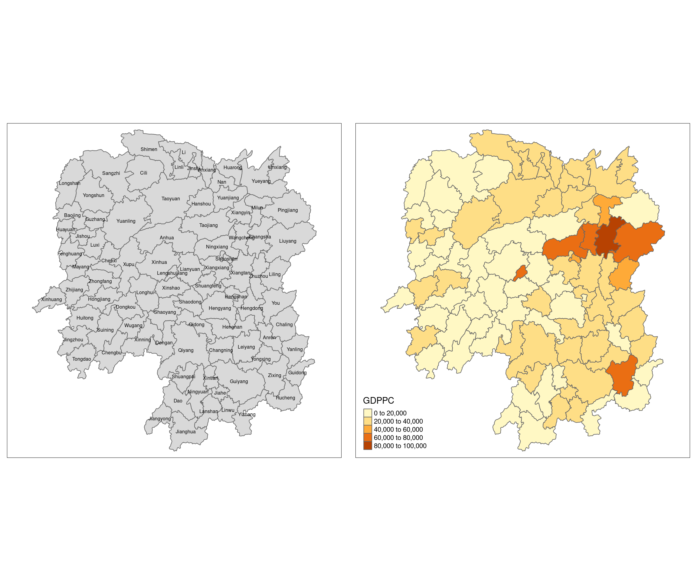
Remember, spatial lag is rarely used to estimate data. It is typically used to derive a clear pattern from existing data.
Computing contiguity weight matrices
In R, the function poly2nb() is part of the spdep package, which is used for spatial data analysis. The poly2nb() function takes in an SFO and creates a neighbor list for a set of spatial polygons. poly2nb() determines which polygons are “neighbors” based on whether they touch each other (contiguity). The output is a neighbor object (class nb) where each polygon is assigned a list of the IDs of its neighboring polygons.
wm_q <- poly2nb(hunan, queen=TRUE)
summary(wm_q)
Neighbour list object:
Number of regions: 88
Number of nonzero links: 448
Percentage nonzero weights: 5.785124
Average number of links: 5.090909
Link number distribution:
1 2 3 4 5 6 7 8 9 11
2 2 12 16 24 14 11 4 2 1
2 least connected regions:
30 65 with 1 link
1 most connected region:
85 with 11 linksThe term “queen” in spatial analysis refers to a method of defining neighborhood relationships between polygons based on how they touch each other. The name comes from the movement of the queen piece in chess, which can move in any direction—horizontally, vertically, or diagonally.
Queen contiguity considers two polygons to be neighbors if they touch at any point, whether they share a full edge (side) or just a corner. This is a broader and more inclusive definition of neighbors compared to rook contiguity.
In rook contiguity, neighbour polygons must share a full edge.
wm_r <- poly2nb(hunan, queen=FALSE)
summary(wm_r)
Neighbour list object:
Number of regions: 88
Number of nonzero links: 440
Percentage nonzero weights: 5.681818
Average number of links: 5
Link number distribution:
1 2 3 4 5 6 7 8 9 10
2 2 12 20 21 14 11 3 2 1
2 least connected regions:
30 65 with 1 link
1 most connected region:
85 with 10 linksThe summary report above shows that there are 88 area units in Hunan. The most connected area unit has 11 neighbours. There are two area units with only one heighbours.
For each polygon in our polygon object, wm_q lists all neighboring polygons. For example, to see the neighbors for the first polygon in the object, type:
wm_q[[1]][1] 2 3 4 57 85We can retrive the county name of Polygon ID=1 by using the code chunk below:
hunan$County[1][1] "Anxiang"To reveal the county names of the five neighboring polygons, the code chunk will be used:
hunan$NAME_3[c(2,3,4,57,85)][1] "Hanshou" "Jinshi" "Li" "Nan" "Taoyuan"We can retrieve the GDPPC (GDP per capita) of these five countries by using the code chunk below.
nb1 <- wm_q[[1]]
nb1 <- hunan$GDPPC[nb1]
nb1
[1] 20981 34592 24473 21311 22879str(wm_q)List of 88
$ : int [1:5] 2 3 4 57 85
$ : int [1:5] 1 57 58 78 85
$ : int [1:4] 1 4 5 85
$ : int [1:4] 1 3 5 6
$ : int [1:4] 3 4 6 85
$ : int [1:5] 4 5 69 75 85
$ : int [1:4] 67 71 74 84
$ : int [1:7] 9 46 47 56 78 80 86
$ : int [1:6] 8 66 68 78 84 86
$ : int [1:8] 16 17 19 20 22 70 72 73
$ : int [1:3] 14 17 72
$ : int [1:5] 13 60 61 63 83
$ : int [1:4] 12 15 60 83
$ : int [1:3] 11 15 17
$ : int [1:4] 13 14 17 83
$ : int [1:5] 10 17 22 72 83
$ : int [1:7] 10 11 14 15 16 72 83
$ : int [1:5] 20 22 23 77 83
$ : int [1:6] 10 20 21 73 74 86
$ : int [1:7] 10 18 19 21 22 23 82
$ : int [1:5] 19 20 35 82 86
$ : int [1:5] 10 16 18 20 83
$ : int [1:7] 18 20 38 41 77 79 82
$ : int [1:5] 25 28 31 32 54
$ : int [1:5] 24 28 31 33 81
$ : int [1:4] 27 33 42 81
$ : int [1:3] 26 29 42
$ : int [1:5] 24 25 33 49 54
$ : int [1:3] 27 37 42
$ : int 33
$ : int [1:8] 24 25 32 36 39 40 56 81
$ : int [1:8] 24 31 50 54 55 56 75 85
$ : int [1:5] 25 26 28 30 81
$ : int [1:3] 36 45 80
$ : int [1:6] 21 41 47 80 82 86
$ : int [1:6] 31 34 40 45 56 80
$ : int [1:4] 29 42 43 44
$ : int [1:4] 23 44 77 79
$ : int [1:5] 31 40 42 43 81
$ : int [1:6] 31 36 39 43 45 79
$ : int [1:6] 23 35 45 79 80 82
$ : int [1:7] 26 27 29 37 39 43 81
$ : int [1:6] 37 39 40 42 44 79
$ : int [1:4] 37 38 43 79
$ : int [1:6] 34 36 40 41 79 80
$ : int [1:3] 8 47 86
$ : int [1:5] 8 35 46 80 86
$ : int [1:5] 50 51 52 53 55
$ : int [1:4] 28 51 52 54
$ : int [1:5] 32 48 52 54 55
$ : int [1:3] 48 49 52
$ : int [1:5] 48 49 50 51 54
$ : int [1:3] 48 55 75
$ : int [1:6] 24 28 32 49 50 52
$ : int [1:5] 32 48 50 53 75
$ : int [1:7] 8 31 32 36 78 80 85
$ : int [1:6] 1 2 58 64 76 85
$ : int [1:5] 2 57 68 76 78
$ : int [1:4] 60 61 87 88
$ : int [1:4] 12 13 59 61
$ : int [1:7] 12 59 60 62 63 77 87
$ : int [1:3] 61 77 87
$ : int [1:4] 12 61 77 83
$ : int [1:2] 57 76
$ : int 76
$ : int [1:5] 9 67 68 76 84
$ : int [1:4] 7 66 76 84
$ : int [1:5] 9 58 66 76 78
$ : int [1:3] 6 75 85
$ : int [1:3] 10 72 73
$ : int [1:3] 7 73 74
$ : int [1:5] 10 11 16 17 70
$ : int [1:5] 10 19 70 71 74
$ : int [1:6] 7 19 71 73 84 86
$ : int [1:6] 6 32 53 55 69 85
$ : int [1:7] 57 58 64 65 66 67 68
$ : int [1:7] 18 23 38 61 62 63 83
$ : int [1:7] 2 8 9 56 58 68 85
$ : int [1:7] 23 38 40 41 43 44 45
$ : int [1:8] 8 34 35 36 41 45 47 56
$ : int [1:6] 25 26 31 33 39 42
$ : int [1:5] 20 21 23 35 41
$ : int [1:9] 12 13 15 16 17 18 22 63 77
$ : int [1:6] 7 9 66 67 74 86
$ : int [1:11] 1 2 3 5 6 32 56 57 69 75 ...
$ : int [1:9] 8 9 19 21 35 46 47 74 84
$ : int [1:4] 59 61 62 88
$ : int [1:2] 59 87
- attr(*, "class")= chr "nb"
- attr(*, "region.id")= chr [1:88] "1" "2" "3" "4" ...
- attr(*, "call")= language poly2nb(pl = hunan, queen = TRUE)
- attr(*, "type")= chr "queen"
- attr(*, "snap")= num 9e-08
- attr(*, "sym")= logi TRUE
- attr(*, "ncomp")=List of 2
..$ nc : num 1
..$ comp.id: num [1:88] 1 1 1 1 1 1 1 1 1 1 ...Visualising contiguity weights
A connectivity graph takes a point and displays a line to each neighboring point. We are working with polygons at the moment, so we will need to get points in order to make our connectivity graphs. The most typically method for this will be polygon centroids. We will calculate these in the sf package before moving onto the graphs.
longitude <- map_dbl(hunan$geometry, ~st_centroid(.x)[[1]])
length(longitude)
[1] 88longitude[1][1] 112.1531latitude <- map_dbl(hunan$geometry, ~st_centroid(.x)[[2]])coords <- cbind(longitude, latitude)head(coords) longitude latitude
[1,] 112.1531 29.44362
[2,] 112.0372 28.86489
[3,] 111.8917 29.47107
[4,] 111.7031 29.74499
[5,] 111.6138 29.49258
[6,] 111.0341 29.79863par(mfrow=c(1,2))
plot(hunan$geometry, border="lightgrey", main="Queen Contiguity")
plot(wm_q, coords, pch = 19, cex = 0.6, add = TRUE, col= "red")
plot(hunan$geometry, border="lightgrey", main="Rook Contiguity")
plot(wm_r, coords, pch = 19, cex = 0.6, add = TRUE, col = "red")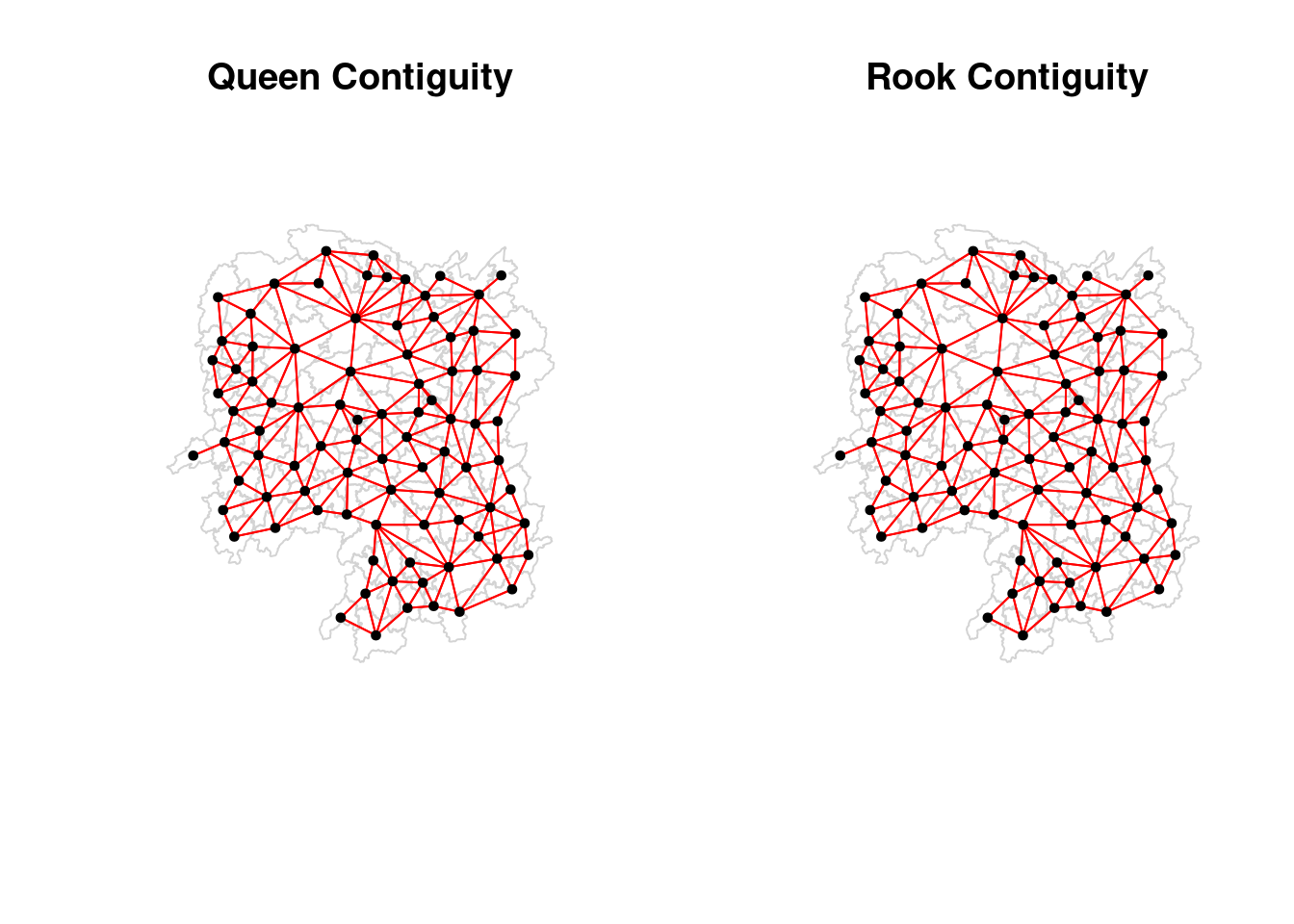
Computing distance based neighbours
In this section, you will learn how to derive distance-based weight matrices by using dnearneigh() of spdep package. The function identifies neighbours of region points by Euclidean distance with a distance band with lower d1= and upper d2= bounds controlled by the bounds= argument. If unprojected coordinates are used and either specified in the coordinates object x or with x as a two column matrix and longlat=TRUE, great circle distances in km will be calculated assuming the WGS84 reference ellipsoid.
Determining the cut-off distance
#coords <- coordinates(hunan)
k1 <- knn2nb(knearneigh(coords))
Warning in knn2nb(knearneigh(coords)): neighbour object has 25 sub-graphsk1dists <- unlist(nbdists(k1, coords, longlat = TRUE))
summary(k1dists) Min. 1st Qu. Median Mean 3rd Qu. Max.
24.79 32.57 38.01 39.07 44.52 61.79 The summary report shows that the largest first nearest neighbour distance is 61.79 km, so using this as the upper threshold gives certainty that all units will have at least one neighbour.
Computing fixed distance weight matrix
Now, we will compute the distance weight matrix by using dnearneigh() as shown in the code chunk below. 0 is the lower bound and 62 is the upper bound of the distance range.
wm_d62 <- dnearneigh(coords, 0, 62, longlat = TRUE)
wm_d62
Neighbour list object:
Number of regions: 88
Number of nonzero links: 324
Percentage nonzero weights: 4.183884
Average number of links: 3.681818 Next, we will use str() to display the content of wm_d62 weight matrix.
str(wm_d62)List of 88
$ : int [1:5] 3 4 5 57 64
$ : int [1:4] 57 58 78 85
$ : int [1:4] 1 4 5 57
$ : int [1:3] 1 3 5
$ : int [1:4] 1 3 4 85
$ : int 69
$ : int [1:2] 67 84
$ : int [1:4] 9 46 47 78
$ : int [1:4] 8 46 68 84
$ : int [1:4] 16 22 70 72
$ : int [1:3] 14 17 72
$ : int [1:5] 13 60 61 63 83
$ : int [1:4] 12 15 60 83
$ : int [1:2] 11 17
$ : int 13
$ : int [1:4] 10 17 22 83
$ : int [1:3] 11 14 16
$ : int [1:3] 20 22 63
$ : int [1:5] 20 21 73 74 82
$ : int [1:5] 18 19 21 22 82
$ : int [1:6] 19 20 35 74 82 86
$ : int [1:4] 10 16 18 20
$ : int [1:3] 41 77 82
$ : int [1:4] 25 28 31 54
$ : int [1:4] 24 28 33 81
$ : int [1:4] 27 33 42 81
$ : int [1:2] 26 29
$ : int [1:6] 24 25 33 49 52 54
$ : int [1:2] 27 37
$ : int 33
$ : int [1:2] 24 36
$ : int 50
$ : int [1:5] 25 26 28 30 81
$ : int [1:3] 36 45 80
$ : int [1:6] 21 41 46 47 80 82
$ : int [1:5] 31 34 45 56 80
$ : int [1:2] 29 42
$ : int [1:3] 44 77 79
$ : int [1:4] 40 42 43 81
$ : int [1:3] 39 45 79
$ : int [1:5] 23 35 45 79 82
$ : int [1:5] 26 37 39 43 81
$ : int [1:3] 39 42 44
$ : int [1:2] 38 43
$ : int [1:6] 34 36 40 41 79 80
$ : int [1:5] 8 9 35 47 86
$ : int [1:5] 8 35 46 80 86
$ : int [1:5] 50 51 52 53 55
$ : int [1:4] 28 51 52 54
$ : int [1:6] 32 48 51 52 54 55
$ : int [1:4] 48 49 50 52
$ : int [1:6] 28 48 49 50 51 54
$ : int [1:2] 48 55
$ : int [1:5] 24 28 49 50 52
$ : int [1:4] 48 50 53 75
$ : int 36
$ : int [1:5] 1 2 3 58 64
$ : int [1:5] 2 57 64 66 68
$ : int [1:3] 60 87 88
$ : int [1:4] 12 13 59 61
$ : int [1:5] 12 60 62 63 87
$ : int [1:4] 61 63 77 87
$ : int [1:5] 12 18 61 62 83
$ : int [1:4] 1 57 58 76
$ : int 76
$ : int [1:5] 58 67 68 76 84
$ : int [1:2] 7 66
$ : int [1:4] 9 58 66 84
$ : int [1:2] 6 75
$ : int [1:3] 10 72 73
$ : int [1:2] 73 74
$ : int [1:3] 10 11 70
$ : int [1:4] 19 70 71 74
$ : int [1:5] 19 21 71 73 86
$ : int [1:2] 55 69
$ : int [1:3] 64 65 66
$ : int [1:3] 23 38 62
$ : int [1:2] 2 8
$ : int [1:4] 38 40 41 45
$ : int [1:5] 34 35 36 45 47
$ : int [1:5] 25 26 33 39 42
$ : int [1:6] 19 20 21 23 35 41
$ : int [1:4] 12 13 16 63
$ : int [1:4] 7 9 66 68
$ : int [1:2] 2 5
$ : int [1:4] 21 46 47 74
$ : int [1:4] 59 61 62 88
$ : int [1:2] 59 87
- attr(*, "class")= chr "nb"
- attr(*, "region.id")= chr [1:88] "1" "2" "3" "4" ...
- attr(*, "call")= language dnearneigh(x = coords, d1 = 0, d2 = 62, longlat = TRUE)
- attr(*, "dnn")= num [1:2] 0 62
- attr(*, "bounds")= chr [1:2] "GE" "LE"
- attr(*, "nbtype")= chr "distance"
- attr(*, "sym")= logi TRUE
- attr(*, "ncomp")=List of 2
..$ nc : num 1
..$ comp.id: num [1:88] 1 1 1 1 1 1 1 1 1 1 ...This returns a list of the indices of nearest neighbours for each point based on a given distance. Don’t worry about the numbers surrounded by square brackets, they just tell you the indexes start from 1 onwards.
This has the problem of a centroid being less effective when the polygon is larger.
Plotting fixed distance weight matrix
par(mfrow=c(1,2))
plot(hunan$geometry, border="lightgrey", main="1st nearest neighbours")
plot(k1, coords, add=TRUE, col="red", length=0.08)
plot(hunan$geometry, border="lightgrey", main="Distance link")
plot(wm_d62, coords, add=TRUE, pch = 19, cex = 0.6)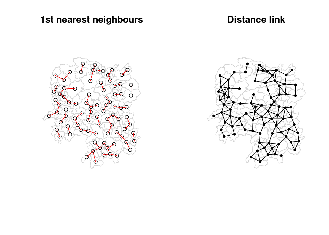
Computing adaptive distance weight matrix
This ensures that each point has a total neighbour count of a certain number. In spatial datasets, points or regions can be distributed unevenly. For instance, urban areas may have many more observations (e.g., people, buildings, events) than rural areas (we’re not just talking about centroids of polygons here). A fixed distance threshold may result in some points having too many neighbors in densely populated areas and too few neighbors in sparsely populated areas. An adaptive distance weight matrix ensures that each point has a consistent number of neighbors, irrespective of the spatial density.
knn6 <- knn2nb(knearneigh(coords, k=6))
knn6
Neighbour list object:
Number of regions: 88
Number of nonzero links: 528
Percentage nonzero weights: 6.818182
Average number of links: 6
Non-symmetric neighbours liststr(knn6)List of 88
$ : int [1:6] 2 3 4 5 57 64
$ : int [1:6] 1 3 57 58 78 85
$ : int [1:6] 1 2 4 5 57 85
$ : int [1:6] 1 3 5 6 69 85
$ : int [1:6] 1 3 4 6 69 85
$ : int [1:6] 3 4 5 69 75 85
$ : int [1:6] 9 66 67 71 74 84
$ : int [1:6] 9 46 47 78 80 86
$ : int [1:6] 8 46 66 68 84 86
$ : int [1:6] 16 19 22 70 72 73
$ : int [1:6] 10 14 16 17 70 72
$ : int [1:6] 13 15 60 61 63 83
$ : int [1:6] 12 15 60 61 63 83
$ : int [1:6] 11 15 16 17 72 83
$ : int [1:6] 12 13 14 17 60 83
$ : int [1:6] 10 11 17 22 72 83
$ : int [1:6] 10 11 14 16 72 83
$ : int [1:6] 20 22 23 63 77 83
$ : int [1:6] 10 20 21 73 74 82
$ : int [1:6] 18 19 21 22 23 82
$ : int [1:6] 19 20 35 74 82 86
$ : int [1:6] 10 16 18 19 20 83
$ : int [1:6] 18 20 41 77 79 82
$ : int [1:6] 25 28 31 52 54 81
$ : int [1:6] 24 28 31 33 54 81
$ : int [1:6] 25 27 29 33 42 81
$ : int [1:6] 26 29 30 37 42 81
$ : int [1:6] 24 25 33 49 52 54
$ : int [1:6] 26 27 37 42 43 81
$ : int [1:6] 26 27 28 33 49 81
$ : int [1:6] 24 25 36 39 40 54
$ : int [1:6] 24 31 50 54 55 56
$ : int [1:6] 25 26 28 30 49 81
$ : int [1:6] 36 40 41 45 56 80
$ : int [1:6] 21 41 46 47 80 82
$ : int [1:6] 31 34 40 45 56 80
$ : int [1:6] 26 27 29 42 43 44
$ : int [1:6] 23 43 44 62 77 79
$ : int [1:6] 25 40 42 43 44 81
$ : int [1:6] 31 36 39 43 45 79
$ : int [1:6] 23 35 45 79 80 82
$ : int [1:6] 26 27 37 39 43 81
$ : int [1:6] 37 39 40 42 44 79
$ : int [1:6] 37 38 39 42 43 79
$ : int [1:6] 34 36 40 41 79 80
$ : int [1:6] 8 9 35 47 78 86
$ : int [1:6] 8 21 35 46 80 86
$ : int [1:6] 49 50 51 52 53 55
$ : int [1:6] 28 33 48 51 52 54
$ : int [1:6] 32 48 51 52 54 55
$ : int [1:6] 28 48 49 50 52 54
$ : int [1:6] 28 48 49 50 51 54
$ : int [1:6] 48 50 51 52 55 75
$ : int [1:6] 24 28 49 50 51 52
$ : int [1:6] 32 48 50 52 53 75
$ : int [1:6] 32 34 36 78 80 85
$ : int [1:6] 1 2 3 58 64 68
$ : int [1:6] 2 57 64 66 68 78
$ : int [1:6] 12 13 60 61 87 88
$ : int [1:6] 12 13 59 61 63 87
$ : int [1:6] 12 13 60 62 63 87
$ : int [1:6] 12 38 61 63 77 87
$ : int [1:6] 12 18 60 61 62 83
$ : int [1:6] 1 3 57 58 68 76
$ : int [1:6] 58 64 66 67 68 76
$ : int [1:6] 9 58 67 68 76 84
$ : int [1:6] 7 65 66 68 76 84
$ : int [1:6] 9 57 58 66 78 84
$ : int [1:6] 4 5 6 32 75 85
$ : int [1:6] 10 16 19 22 72 73
$ : int [1:6] 7 19 73 74 84 86
$ : int [1:6] 10 11 14 16 17 70
$ : int [1:6] 10 19 21 70 71 74
$ : int [1:6] 19 21 71 73 84 86
$ : int [1:6] 6 32 50 53 55 69
$ : int [1:6] 58 64 65 66 67 68
$ : int [1:6] 18 23 38 61 62 63
$ : int [1:6] 2 8 9 46 58 68
$ : int [1:6] 38 40 41 43 44 45
$ : int [1:6] 34 35 36 41 45 47
$ : int [1:6] 25 26 28 33 39 42
$ : int [1:6] 19 20 21 23 35 41
$ : int [1:6] 12 13 15 16 22 63
$ : int [1:6] 7 9 66 68 71 74
$ : int [1:6] 2 3 4 5 56 69
$ : int [1:6] 8 9 21 46 47 74
$ : int [1:6] 59 60 61 62 63 88
$ : int [1:6] 59 60 61 62 63 87
- attr(*, "region.id")= chr [1:88] "1" "2" "3" "4" ...
- attr(*, "call")= language knearneigh(x = coords, k = 6)
- attr(*, "sym")= logi FALSE
- attr(*, "type")= chr "knn"
- attr(*, "knn-k")= num 6
- attr(*, "class")= chr "nb"
- attr(*, "ncomp")=List of 2
..$ nc : num 1
..$ comp.id: num [1:88] 1 1 1 1 1 1 1 1 1 1 ...Weights based on Inverse Distance Weighting (IDW)
It estimates the value at an unknown location based on the values at nearby known locations, with the assumption that points that are closer to the unknown location have more influence than points that are farther away.
dist <- nbdists(wm_q, coords, longlat = TRUE)
ids <- lapply(dist, function(x) 1/(x))
ids
[[1]]
[1] 0.01535405 0.03916350 0.01820896 0.02807922 0.01145113
[[2]]
[1] 0.01535405 0.01764308 0.01925924 0.02323898 0.01719350
[[3]]
[1] 0.03916350 0.02822040 0.03695795 0.01395765
[[4]]
[1] 0.01820896 0.02822040 0.03414741 0.01539065
[[5]]
[1] 0.03695795 0.03414741 0.01524598 0.01618354
[[6]]
[1] 0.015390649 0.015245977 0.021748129 0.011883901 0.009810297
[[7]]
[1] 0.01708612 0.01473997 0.01150924 0.01872915
[[8]]
[1] 0.02022144 0.03453056 0.02529256 0.01036340 0.02284457 0.01500600 0.01515314
[[9]]
[1] 0.02022144 0.01574888 0.02109502 0.01508028 0.02902705 0.01502980
[[10]]
[1] 0.02281552 0.01387777 0.01538326 0.01346650 0.02100510 0.02631658 0.01874863
[8] 0.01500046
[[11]]
[1] 0.01882869 0.02243492 0.02247473
[[12]]
[1] 0.02779227 0.02419652 0.02333385 0.02986130 0.02335429
[[13]]
[1] 0.02779227 0.02650020 0.02670323 0.01714243
[[14]]
[1] 0.01882869 0.01233868 0.02098555
[[15]]
[1] 0.02650020 0.01233868 0.01096284 0.01562226
[[16]]
[1] 0.02281552 0.02466962 0.02765018 0.01476814 0.01671430
[[17]]
[1] 0.01387777 0.02243492 0.02098555 0.01096284 0.02466962 0.01593341 0.01437996
[[18]]
[1] 0.02039779 0.02032767 0.01481665 0.01473691 0.01459380
[[19]]
[1] 0.01538326 0.01926323 0.02668415 0.02140253 0.01613589 0.01412874
[[20]]
[1] 0.01346650 0.02039779 0.01926323 0.01723025 0.02153130 0.01469240 0.02327034
[[21]]
[1] 0.02668415 0.01723025 0.01766299 0.02644986 0.02163800
[[22]]
[1] 0.02100510 0.02765018 0.02032767 0.02153130 0.01489296
[[23]]
[1] 0.01481665 0.01469240 0.01401432 0.02246233 0.01880425 0.01530458 0.01849605
[[24]]
[1] 0.02354598 0.01837201 0.02607264 0.01220154 0.02514180
[[25]]
[1] 0.02354598 0.02188032 0.01577283 0.01949232 0.02947957
[[26]]
[1] 0.02155798 0.01745522 0.02212108 0.02220532
[[27]]
[1] 0.02155798 0.02490625 0.01562326
[[28]]
[1] 0.01837201 0.02188032 0.02229549 0.03076171 0.02039506
[[29]]
[1] 0.02490625 0.01686587 0.01395022
[[30]]
[1] 0.02090587
[[31]]
[1] 0.02607264 0.01577283 0.01219005 0.01724850 0.01229012 0.01609781 0.01139438
[8] 0.01150130
[[32]]
[1] 0.01220154 0.01219005 0.01712515 0.01340413 0.01280928 0.01198216 0.01053374
[8] 0.01065655
[[33]]
[1] 0.01949232 0.01745522 0.02229549 0.02090587 0.01979045
[[34]]
[1] 0.03113041 0.03589551 0.02882915
[[35]]
[1] 0.01766299 0.02185795 0.02616766 0.02111721 0.02108253 0.01509020
[[36]]
[1] 0.01724850 0.03113041 0.01571707 0.01860991 0.02073549 0.01680129
[[37]]
[1] 0.01686587 0.02234793 0.01510990 0.01550676
[[38]]
[1] 0.01401432 0.02407426 0.02276151 0.01719415
[[39]]
[1] 0.01229012 0.02172543 0.01711924 0.02629732 0.01896385
[[40]]
[1] 0.01609781 0.01571707 0.02172543 0.01506473 0.01987922 0.01894207
[[41]]
[1] 0.02246233 0.02185795 0.02205991 0.01912542 0.01601083 0.01742892
[[42]]
[1] 0.02212108 0.01562326 0.01395022 0.02234793 0.01711924 0.01836831 0.01683518
[[43]]
[1] 0.01510990 0.02629732 0.01506473 0.01836831 0.03112027 0.01530782
[[44]]
[1] 0.01550676 0.02407426 0.03112027 0.01486508
[[45]]
[1] 0.03589551 0.01860991 0.01987922 0.02205991 0.02107101 0.01982700
[[46]]
[1] 0.03453056 0.04033752 0.02689769
[[47]]
[1] 0.02529256 0.02616766 0.04033752 0.01949145 0.02181458
[[48]]
[1] 0.02313819 0.03370576 0.02289485 0.01630057 0.01818085
[[49]]
[1] 0.03076171 0.02138091 0.02394529 0.01990000
[[50]]
[1] 0.01712515 0.02313819 0.02551427 0.02051530 0.02187179
[[51]]
[1] 0.03370576 0.02138091 0.02873854
[[52]]
[1] 0.02289485 0.02394529 0.02551427 0.02873854 0.03516672
[[53]]
[1] 0.01630057 0.01979945 0.01253977
[[54]]
[1] 0.02514180 0.02039506 0.01340413 0.01990000 0.02051530 0.03516672
[[55]]
[1] 0.01280928 0.01818085 0.02187179 0.01979945 0.01882298
[[56]]
[1] 0.01036340 0.01139438 0.01198216 0.02073549 0.01214479 0.01362855 0.01341697
[[57]]
[1] 0.028079221 0.017643082 0.031423501 0.029114131 0.013520292 0.009903702
[[58]]
[1] 0.01925924 0.03142350 0.02722997 0.01434859 0.01567192
[[59]]
[1] 0.01696711 0.01265572 0.01667105 0.01785036
[[60]]
[1] 0.02419652 0.02670323 0.01696711 0.02343040
[[61]]
[1] 0.02333385 0.01265572 0.02343040 0.02514093 0.02790764 0.01219751 0.02362452
[[62]]
[1] 0.02514093 0.02002219 0.02110260
[[63]]
[1] 0.02986130 0.02790764 0.01407043 0.01805987
[[64]]
[1] 0.02911413 0.01689892
[[65]]
[1] 0.02471705
[[66]]
[1] 0.01574888 0.01726461 0.03068853 0.01954805 0.01810569
[[67]]
[1] 0.01708612 0.01726461 0.01349843 0.01361172
[[68]]
[1] 0.02109502 0.02722997 0.03068853 0.01406357 0.01546511
[[69]]
[1] 0.02174813 0.01645838 0.01419926
[[70]]
[1] 0.02631658 0.01963168 0.02278487
[[71]]
[1] 0.01473997 0.01838483 0.03197403
[[72]]
[1] 0.01874863 0.02247473 0.01476814 0.01593341 0.01963168
[[73]]
[1] 0.01500046 0.02140253 0.02278487 0.01838483 0.01652709
[[74]]
[1] 0.01150924 0.01613589 0.03197403 0.01652709 0.01342099 0.02864567
[[75]]
[1] 0.011883901 0.010533736 0.012539774 0.018822977 0.016458383 0.008217581
[[76]]
[1] 0.01352029 0.01434859 0.01689892 0.02471705 0.01954805 0.01349843 0.01406357
[[77]]
[1] 0.014736909 0.018804247 0.022761507 0.012197506 0.020022195 0.014070428
[7] 0.008440896
[[78]]
[1] 0.02323898 0.02284457 0.01508028 0.01214479 0.01567192 0.01546511 0.01140779
[[79]]
[1] 0.01530458 0.01719415 0.01894207 0.01912542 0.01530782 0.01486508 0.02107101
[[80]]
[1] 0.01500600 0.02882915 0.02111721 0.01680129 0.01601083 0.01982700 0.01949145
[8] 0.01362855
[[81]]
[1] 0.02947957 0.02220532 0.01150130 0.01979045 0.01896385 0.01683518
[[82]]
[1] 0.02327034 0.02644986 0.01849605 0.02108253 0.01742892
[[83]]
[1] 0.023354289 0.017142433 0.015622258 0.016714303 0.014379961 0.014593799
[7] 0.014892965 0.018059871 0.008440896
[[84]]
[1] 0.01872915 0.02902705 0.01810569 0.01361172 0.01342099 0.01297994
[[85]]
[1] 0.011451133 0.017193502 0.013957649 0.016183544 0.009810297 0.010656545
[7] 0.013416965 0.009903702 0.014199260 0.008217581 0.011407794
[[86]]
[1] 0.01515314 0.01502980 0.01412874 0.02163800 0.01509020 0.02689769 0.02181458
[8] 0.02864567 0.01297994
[[87]]
[1] 0.01667105 0.02362452 0.02110260 0.02058034
[[88]]
[1] 0.01785036 0.02058034function(x) 1/(x): This function takes each vector of distances (x) from the list dist and computes the inverse of those distances (i.e., 1 / distance).
- The result of applying this function is that points closer to each other will have a larger value (since the inverse of a small distance is large), and points farther away will have smaller values.
lapply(): This function applies a given function to each element of a list (dist in this case). It loops over each element of the list and applies the specified function.
The result (ids) will be a list where each element contains the inverse distances between a point and its neighbors.
Knowing the inverse distances alone isn’t inherently useful unless you are applying them for a specific purpose in spatial analysis. The inverse distance is typically used as a weight in various spatial models or techniques, where closer points have more influence than distant ones. One drawback is that this method does not do edge correction, which means that points around the edges will have less neighbours and hence lower values.
rswm_q <- nb2listw(wm_q, style="W", zero.policy = TRUE)
rswm_q
Characteristics of weights list object:
Neighbour list object:
Number of regions: 88
Number of nonzero links: 448
Percentage nonzero weights: 5.785124
Average number of links: 5.090909
Weights style: W
Weights constants summary:
n nn S0 S1 S2
W 88 7744 88 37.86334 365.9147To see the weight of the first polygon’s eight neighbors type:
rswm_q$weights[10][[1]]
[1] 0.125 0.125 0.125 0.125 0.125 0.125 0.125 0.125Each neighbor is assigned a 0.125 of the total weight. This means that when R computes the average neighboring income values, each neighbor’s income will be multiplied by 0.125 before being tallied.
library(spdep)

# Example: coords is your matrix of known point coordinates
# values contains the known values (e.g., temperature, pollution, etc.)
# x_0 is the location where you want to estimate the value
x_0 <- c(lon, lat)  # coordinates of the unknown point

# Calculate the distances between the unknown point and known points
distances <- spDistsN1(coords, x_0, longlat = TRUE)

# Set the power parameter for inverse distance (usually 2)
p <- 2

# Calculate inverse distances (weights)
weights <- 1 / (distances^p)

# Estimate the value at x_0 by calculating the weighted average
estimated_value <- sum(weights * values) / sum(weights)

# Print the estimated value
print(estimated_value)
“W” stands for row-standardized weights. This means that the weights for each row (i.e., for each observation or spatial point) are normalized so that they sum up to 1. In a row-standardized weight matrix, each element is divided by the sum of the weights for that row, ensuring that all the weights for a given point’s neighbors add up to 1.
Row-standardization is useful when you want to make the sum of weights comparable across observations. It helps in cases where some points have many neighbors and others have few, so you ensure that every point contributes equally overall.
“B” stands for binary weights. In this case, each neighbor is either given a weight of 1 (if it is a neighbor) or 0 (if it is not a neighbor). Binary weights are the simplest form of spatial weighting. Each point either has full influence on its neighbors (weight = 1), or no influence (weight = 0), without considering the distance or the number of neighbors. Binary weights are useful in cases where you are only interested in whether two points are neighbors, without differentiating between them based on distance or proximity. It is a straightforward approach for identifying and analyzing neighborhood structures. All neighbors have the same influence, regardless of how many neighbors exist or how far apart they are.
zero.policy = TRUE: This allows handling cases where some points have no neighbors. If zero.policy = TRUE, the function will handle these cases by assigning zero weights to points with no neighbors, instead of causing an error.
This alone will not give you an estimate of a value given a location. For that, you’ll need spatial lagged models.
Application of Spatial Weight Matrix
In this section, you will learn how to create four different spatial lagged variables. A spatial lagged model is where the value at a given point is influenced by a weighted average of the values of its neighbors.
Spatial lag with row-standardised weights
Computing the average neighbor GDPPC value for each polygon.
GDPPC.lag <- lag.listw(rswm_q, hunan$GDPPC)
GDPPC.lag
[1] 24847.20 22724.80 24143.25 27737.50 27270.25 21248.80 43747.00 33582.71
[9] 45651.17 32027.62 32671.00 20810.00 25711.50 30672.33 33457.75 31689.20
[17] 20269.00 23901.60 25126.17 21903.43 22718.60 25918.80 20307.00 20023.80
[25] 16576.80 18667.00 14394.67 19848.80 15516.33 20518.00 17572.00 15200.12
[33] 18413.80 14419.33 24094.50 22019.83 12923.50 14756.00 13869.80 12296.67
[41] 15775.17 14382.86 11566.33 13199.50 23412.00 39541.00 36186.60 16559.60
[49] 20772.50 19471.20 19827.33 15466.80 12925.67 18577.17 14943.00 24913.00
[57] 25093.00 24428.80 17003.00 21143.75 20435.00 17131.33 24569.75 23835.50
[65] 26360.00 47383.40 55157.75 37058.00 21546.67 23348.67 42323.67 28938.60
[73] 25880.80 47345.67 18711.33 29087.29 20748.29 35933.71 15439.71 29787.50
[81] 18145.00 21617.00 29203.89 41363.67 22259.09 44939.56 16902.00 16930.00Each number correspond to each row in hunan.
We can append the spatially lag GDPPC values onto hunan sf data frame by using the code chunk below.
lag.list <- list(hunan$NAME_3, lag.listw(rswm_q, hunan$GDPPC))
lag.res <- as.data.frame(lag.list)
colnames(lag.res) <- c("NAME_3", "lag GDPPC")
hunan <- left_join(hunan,lag.res)
Joining with `by = join_by(NAME_3)`The following table shows the average neighboring income values (stored in the Inc.lag object) for each county.
head(hunan)Simple feature collection with 6 features and 36 fields
Geometry type: POLYGON
Dimension: XY
Bounding box: xmin: 110.4922 ymin: 28.61762 xmax: 112.3013 ymax: 30.12812
Geodetic CRS: WGS 84
NAME_2 ID_3 NAME_3 ENGTYPE_3 Shape_Leng Shape_Area County City
1 Changde 21098 Anxiang County 1.869074 0.10056190 Anxiang Changde
2 Changde 21100 Hanshou County 2.360691 0.19978745 Hanshou Changde
3 Changde 21101 Jinshi County City 1.425620 0.05302413 Jinshi Changde
4 Changde 21102 Li County 3.474325 0.18908121 Li Changde
5 Changde 21103 Linli County 2.289506 0.11450357 Linli Changde
6 Changde 21104 Shimen County 4.171918 0.37194707 Shimen Changde
avg_wage deposite FAI Gov_Rev Gov_Exp GDP GDPPC GIO Loan NIPCR
1 31935 5517.2 3541.0 243.64 1779.5 12482.0 23667 5108.9 2806.9 7693.7
2 32265 7979.0 8665.0 386.13 2062.4 15788.0 20981 13491.0 4550.0 8269.9
3 28692 4581.7 4777.0 373.31 1148.4 8706.9 34592 10935.0 2242.0 8169.9
4 32541 13487.0 16066.0 709.61 2459.5 20322.0 24473 18402.0 6748.0 8377.0
5 32667 564.1 7781.2 336.86 1538.7 10355.0 25554 8214.0 358.0 8143.1
6 33261 8334.4 10531.0 548.33 2178.8 16293.0 27137 17795.0 6026.5 6156.0
Bed Emp EmpR EmpRT Pri_Stu Sec_Stu Household Household_R NOIP Pop_R
1 1931 336.39 270.5 205.9 19.584 17.819 148.1 135.4 53 346.0
2 2560 456.78 388.8 246.7 42.097 33.029 240.2 208.7 95 553.2
3 848 122.78 82.1 61.7 8.723 7.592 81.9 43.7 77 92.4
4 2038 513.44 426.8 227.1 38.975 33.938 268.5 256.0 96 539.7
5 1440 307.36 272.2 100.8 23.286 18.943 129.1 157.2 99 246.6
6 2502 392.05 329.6 193.8 29.245 26.104 190.6 184.7 122 399.2
RSCG Pop_T Agri Service Disp_Inc RORP ROREmp lag GDPPC
1 3957.9 528.3 4524.41 14100 16610 0.6549309 0.8041262 24847.20
2 4460.5 804.6 6545.35 17727 18925 0.6875466 0.8511756 22724.80
3 3683.0 251.8 2562.46 7525 19498 0.3669579 0.6686757 24143.25
4 7110.2 832.5 7562.34 53160 18985 0.6482883 0.8312558 27737.50
5 3604.9 409.3 3583.91 7031 18604 0.6024921 0.8856065 27270.25
6 6490.7 600.5 5266.51 6981 19275 0.6647794 0.8407091 21248.80
geometry
1 POLYGON ((112.0625 29.75523...
2 POLYGON ((112.2288 29.11684...
3 POLYGON ((111.8927 29.6013,...
4 POLYGON ((111.3731 29.94649...
5 POLYGON ((111.6324 29.76288...
6 POLYGON ((110.8825 30.11675...Next, we will plot both the GDPPC and spatial lag GDPPC for comparison using the code chunk below.
gdppc <- qtm(hunan, "GDPPC")
lag_gdppc <- qtm(hunan, "lag GDPPC")
tmap_arrange(gdppc, lag_gdppc, asp=1, ncol=2)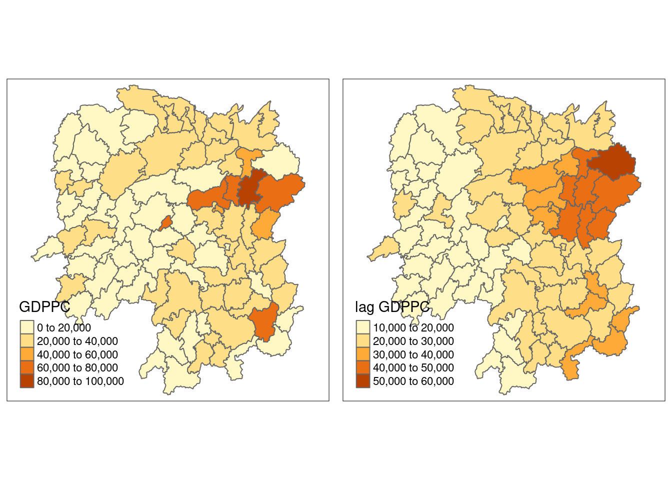
Spatial lag as a sum of neighbouring values
b_weights <- lapply(wm_q, function(x) 0*x + 1)
b_weights2 <- nb2listw(wm_q,
                       glist = b_weights,
                       style = "B")
b_weights2
Characteristics of weights list object:
Neighbour list object:
Number of regions: 88
Number of nonzero links: 448
Percentage nonzero weights: 5.785124
Average number of links: 5.090909
Weights style: B
Weights constants summary:
n nn S0 S1 S2
B 88 7744 448 896 10224lag_sum <- list(hunan$NAME_3, lag.listw(b_weights2, hunan$GDPPC))
lag.res <- as.data.frame(lag_sum)
colnames(lag.res) <- c("NAME_3", "lag_sum GDPPC")hunan <- left_join(hunan, lag.res)Joining with `by = join_by(NAME_3)`gdppc <- qtm(hunan, "GDPPC")
lag_sum_gdppc <- qtm(hunan, "lag_sum GDPPC")
tmap_arrange(gdppc, lag_sum_gdppc, asp=1, ncol=2)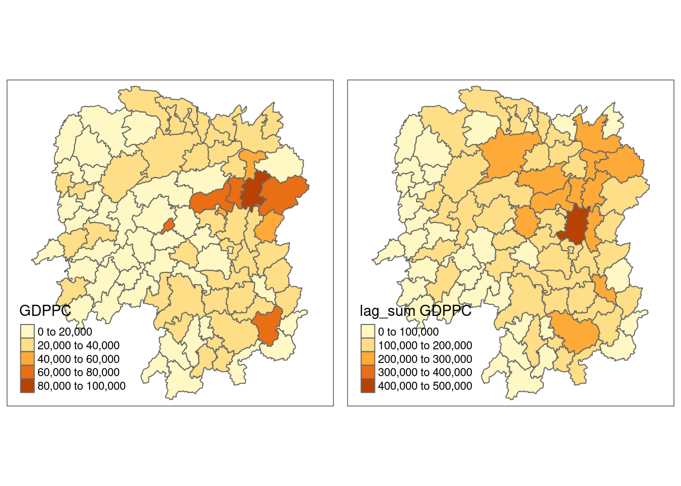
Spatial window average
The spatial window average uses row-standardized weights and includes the diagonal element. To do this in R, we need to go back to the neighbors structure and add the diagonal element before assigning weights.
To add the diagonal element to the neighbour list, we just need to use include.self() from spdep.
wm_qs <- include.self(wm_q)
wm_qs[[1]]
[1] 1 2 3 4 57 85Now we obtain weights with nb2listw():
wm_qs <- nb2listw(wm_qs)
wm_qs
Characteristics of weights list object:
Neighbour list object:
Number of regions: 88
Number of nonzero links: 536
Percentage nonzero weights: 6.921488
Average number of links: 6.090909
Weights style: W
Weights constants summary:
n nn S0 S1 S2
W 88 7744 88 30.90265 357.5308Lastly, we just need to create the lag variable from our weight structure and GDPPC variable.
lag_w_avg_gpdpc <- lag.listw(wm_qs,
                             hunan$GDPPC)
lag_w_avg_gpdpc
[1] 24650.50 22434.17 26233.00 27084.60 26927.00 22230.17 47621.20 37160.12
[9] 49224.71 29886.89 26627.50 22690.17 25366.40 25825.75 30329.00 32682.83
[17] 25948.62 23987.67 25463.14 21904.38 23127.50 25949.83 20018.75 19524.17
[25] 18955.00 17800.40 15883.00 18831.33 14832.50 17965.00 17159.89 16199.44
[33] 18764.50 26878.75 23188.86 20788.14 12365.20 15985.00 13764.83 11907.43
[41] 17128.14 14593.62 11644.29 12706.00 21712.29 43548.25 35049.00 16226.83
[49] 19294.40 18156.00 19954.75 18145.17 12132.75 18419.29 14050.83 23619.75
[57] 24552.71 24733.67 16762.60 20932.60 19467.75 18334.00 22541.00 26028.00
[65] 29128.50 46569.00 47576.60 36545.50 20838.50 22531.00 42115.50 27619.00
[73] 27611.33 44523.29 18127.43 28746.38 20734.50 33880.62 14716.38 28516.22
[81] 18086.14 21244.50 29568.80 48119.71 22310.75 43151.60 17133.40 17009.33Next, we will convert the lag variable listw object into a data.frame by using as.data.frame().
lag.list.wm_qs <- list(hunan$NAME_3, lag.listw(wm_qs, hunan$GDPPC))
lag_wm_qs.res <- as.data.frame(lag.list.wm_qs)
colnames(lag_wm_qs.res) <- c("NAME_3", "lag_window_avg GDPPC")
Next, the code chunk below will be used to append lag_window_avg GDPPC values onto hunan sf data.frame by using left_join() of dplyr package.
hunan <- left_join(hunan, lag_wm_qs.res)Joining with `by = join_by(NAME_3)`To compare the values of lag GDPPC and Spatial window average, kable() of Knitr package is used to prepare a table using the code chunk below.
pacman::p_load(knitr)hunan %>%
select("County",
"lag GDPPC",
"lag_window_avg GDPPC") %>%
kable()| County | lag GDPPC | lag_window_avg GDPPC | geometry |
|---|---|---|---|
| Anxiang | 24847.20 | 24650.50 | POLYGON ((112.0625 29.75523… |
| Hanshou | 22724.80 | 22434.17 | POLYGON ((112.2288 29.11684… |
| Jinshi | 24143.25 | 26233.00 | POLYGON ((111.8927 29.6013,… |
| Li | 27737.50 | 27084.60 | POLYGON ((111.3731 29.94649… |
| Linli | 27270.25 | 26927.00 | POLYGON ((111.6324 29.76288… |
| Shimen | 21248.80 | 22230.17 | POLYGON ((110.8825 30.11675… |
| Liuyang | 43747.00 | 47621.20 | POLYGON ((113.9905 28.5682,… |
| Ningxiang | 33582.71 | 37160.12 | POLYGON ((112.7181 28.38299… |
| Wangcheng | 45651.17 | 49224.71 | POLYGON ((112.7914 28.52688… |
| Anren | 32027.62 | 29886.89 | POLYGON ((113.1757 26.82734… |
| Guidong | 32671.00 | 26627.50 | POLYGON ((114.1799 26.20117… |
| Jiahe | 20810.00 | 22690.17 | POLYGON ((112.4425 25.74358… |
| Linwu | 25711.50 | 25366.40 | POLYGON ((112.5914 25.55143… |
| Rucheng | 30672.33 | 25825.75 | POLYGON ((113.6759 25.87578… |
| Yizhang | 33457.75 | 30329.00 | POLYGON ((113.2621 25.68394… |
| Yongxing | 31689.20 | 32682.83 | POLYGON ((113.3169 26.41843… |
| Zixing | 20269.00 | 25948.62 | POLYGON ((113.7311 26.16259… |
| Changning | 23901.60 | 23987.67 | POLYGON ((112.6144 26.60198… |
| Hengdong | 25126.17 | 25463.14 | POLYGON ((113.1056 27.21007… |
| Hengnan | 21903.43 | 21904.38 | POLYGON ((112.7599 26.98149… |
| Hengshan | 22718.60 | 23127.50 | POLYGON ((112.607 27.4689, … |
| Leiyang | 25918.80 | 25949.83 | POLYGON ((112.9996 26.69276… |
| Qidong | 20307.00 | 20018.75 | POLYGON ((111.7818 27.0383,… |
| Chenxi | 20023.80 | 19524.17 | POLYGON ((110.2624 28.21778… |
| Zhongfang | 16576.80 | 18955.00 | POLYGON ((109.9431 27.72858… |
| Huitong | 18667.00 | 17800.40 | POLYGON ((109.9419 27.10512… |
| Jingzhou | 14394.67 | 15883.00 | POLYGON ((109.8186 26.75842… |
| Mayang | 19848.80 | 18831.33 | POLYGON ((109.795 27.98008,… |
| Tongdao | 15516.33 | 14832.50 | POLYGON ((109.9294 26.46561… |
| Xinhuang | 20518.00 | 17965.00 | POLYGON ((109.227 27.43733,… |
| Xupu | 17572.00 | 17159.89 | POLYGON ((110.7189 28.30485… |
| Yuanling | 15200.12 | 16199.44 | POLYGON ((110.9652 28.99895… |
| Zhijiang | 18413.80 | 18764.50 | POLYGON ((109.8818 27.60661… |
| Lengshuijiang | 14419.33 | 26878.75 | POLYGON ((111.5307 27.81472… |
| Shuangfeng | 24094.50 | 23188.86 | POLYGON ((112.263 27.70421,… |
| Xinhua | 22019.83 | 20788.14 | POLYGON ((111.3345 28.19642… |
| Chengbu | 12923.50 | 12365.20 | POLYGON ((110.4455 26.69317… |
| Dongan | 14756.00 | 15985.00 | POLYGON ((111.4531 26.86812… |
| Dongkou | 13869.80 | 13764.83 | POLYGON ((110.6622 27.37305… |
| Longhui | 12296.67 | 11907.43 | POLYGON ((110.985 27.65983,… |
| Shaodong | 15775.17 | 17128.14 | POLYGON ((111.9054 27.40254… |
| Suining | 14382.86 | 14593.62 | POLYGON ((110.389 27.10006,… |
| Wugang | 11566.33 | 11644.29 | POLYGON ((110.9878 27.03345… |
| Xinning | 13199.50 | 12706.00 | POLYGON ((111.0736 26.84627… |
| Xinshao | 23412.00 | 21712.29 | POLYGON ((111.6013 27.58275… |
| Shaoshan | 39541.00 | 43548.25 | POLYGON ((112.5391 27.97742… |
| Xiangxiang | 36186.60 | 35049.00 | POLYGON ((112.4549 28.05783… |
| Baojing | 16559.60 | 16226.83 | POLYGON ((109.7015 28.82844… |
| Fenghuang | 20772.50 | 19294.40 | POLYGON ((109.5239 28.19206… |
| Guzhang | 19471.20 | 18156.00 | POLYGON ((109.8968 28.74034… |
| Huayuan | 19827.33 | 19954.75 | POLYGON ((109.5647 28.61712… |
| Jishou | 15466.80 | 18145.17 | POLYGON ((109.8375 28.4696,… |
| Longshan | 12925.67 | 12132.75 | POLYGON ((109.6337 29.62521… |
| Luxi | 18577.17 | 18419.29 | POLYGON ((110.1067 28.41835… |
| Yongshun | 14943.00 | 14050.83 | POLYGON ((110.0003 29.29499… |
| Anhua | 24913.00 | 23619.75 | POLYGON ((111.6034 28.63716… |
| Nan | 25093.00 | 24552.71 | POLYGON ((112.3232 29.46074… |
| Yuanjiang | 24428.80 | 24733.67 | POLYGON ((112.4391 29.1791,… |
| Jianghua | 17003.00 | 16762.60 | POLYGON ((111.6461 25.29661… |
| Lanshan | 21143.75 | 20932.60 | POLYGON ((112.2286 25.61123… |
| Ningyuan | 20435.00 | 19467.75 | POLYGON ((112.0715 26.09892… |
| Shuangpai | 17131.33 | 18334.00 | POLYGON ((111.8864 26.11957… |
| Xintian | 24569.75 | 22541.00 | POLYGON ((112.2578 26.0796,… |
| Huarong | 23835.50 | 26028.00 | POLYGON ((112.9242 29.69134… |
| Linxiang | 26360.00 | 29128.50 | POLYGON ((113.5502 29.67418… |
| Miluo | 47383.40 | 46569.00 | POLYGON ((112.9902 29.02139… |
| Pingjiang | 55157.75 | 47576.60 | POLYGON ((113.8436 29.06152… |
| Xiangyin | 37058.00 | 36545.50 | POLYGON ((112.9173 28.98264… |
| Cili | 21546.67 | 20838.50 | POLYGON ((110.8822 29.69017… |
| Chaling | 23348.67 | 22531.00 | POLYGON ((113.7666 27.10573… |
| Liling | 42323.67 | 42115.50 | POLYGON ((113.5673 27.94346… |
| Yanling | 28938.60 | 27619.00 | POLYGON ((113.9292 26.6154,… |
| You | 25880.80 | 27611.33 | POLYGON ((113.5879 27.41324… |
| Zhuzhou | 47345.67 | 44523.29 | POLYGON ((113.2493 28.02411… |
| Sangzhi | 18711.33 | 18127.43 | POLYGON ((110.556 29.40543,… |
| Yueyang | 29087.29 | 28746.38 | POLYGON ((113.343 29.61064,… |
| Qiyang | 20748.29 | 20734.50 | POLYGON ((111.5563 26.81318… |
| Taojiang | 35933.71 | 33880.62 | POLYGON ((112.0508 28.67265… |
| Shaoyang | 15439.71 | 14716.38 | POLYGON ((111.5013 27.30207… |
| Lianyuan | 29787.50 | 28516.22 | POLYGON ((111.6789 28.02946… |
| Hongjiang | 18145.00 | 18086.14 | POLYGON ((110.1441 27.47513… |
| Hengyang | 21617.00 | 21244.50 | POLYGON ((112.7144 26.98613… |
| Guiyang | 29203.89 | 29568.80 | POLYGON ((113.0811 26.04963… |
| Changsha | 41363.67 | 48119.71 | POLYGON ((112.9421 28.03722… |
| Taoyuan | 22259.09 | 22310.75 | POLYGON ((112.0612 29.32855… |
| Xiangtan | 44939.56 | 43151.60 | POLYGON ((113.0426 27.8942,… |
| Dao | 16902.00 | 17133.40 | POLYGON ((111.498 25.81679,… |
| Jiangyong | 16930.00 | 17009.33 | POLYGON ((111.3659 25.39472… |
Lastly, qtm() of tmap package is used to plot the lag_gdppc and w_ave_gdppc maps next to each other for quick comparison.
w_avg_gdppc <- qtm(hunan, "lag_window_avg GDPPC")
tmap_arrange(lag_gdppc, w_avg_gdppc, asp=1, ncol=2)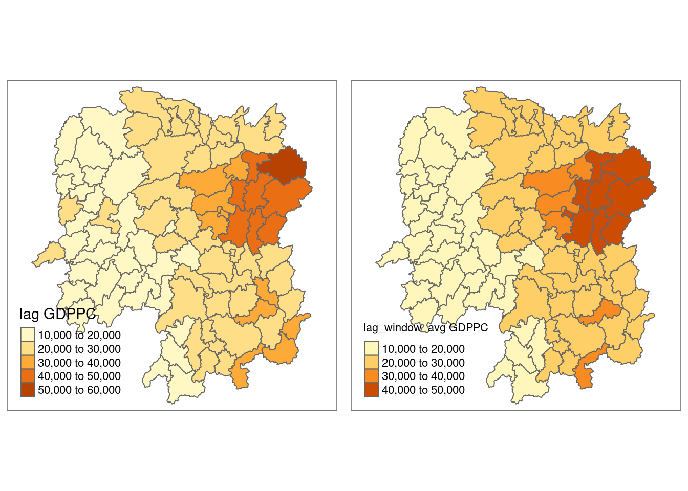
Spatial window sum
The spatial window sum is the counterpart of the window average, but without using row-standardized weights.
wm_qs <- include.self(wm_q)
wm_qs
Neighbour list object:
Number of regions: 88
Number of nonzero links: 536
Percentage nonzero weights: 6.921488
Average number of links: 6.090909 Next, we will assign binary weights to the neighbour structure that includes the diagonal element.
b_weights <- lapply(wm_qs, function(x) 0*x + 1)
b_weights[1][[1]]
[1] 1 1 1 1 1 1Again, we use nb2listw() and glist() to explicitly assign weight values.
b_weights2 <- nb2listw(wm_qs,
glist = b_weights,
style = "B")
b_weights2Characteristics of weights list object:
Neighbour list object:
Number of regions: 88
Number of nonzero links: 536
Percentage nonzero weights: 6.921488
Average number of links: 6.090909
Weights style: B
Weights constants summary:
n nn S0 S1 S2
B 88 7744 536 1072 14160With our new weight structure, we can compute the lag variable with lag.listw().
w_sum_gdppc <- list(hunan$NAME_3, lag.listw(b_weights2, hunan$GDPPC))
w_sum_gdppc
[[1]]
[1] "Anxiang" "Hanshou" "Jinshi" "Li"
[5] "Linli" "Shimen" "Liuyang" "Ningxiang"
[9] "Wangcheng" "Anren" "Guidong" "Jiahe"
[13] "Linwu" "Rucheng" "Yizhang" "Yongxing"
[17] "Zixing" "Changning" "Hengdong" "Hengnan"
[21] "Hengshan" "Leiyang" "Qidong" "Chenxi"
[25] "Zhongfang" "Huitong" "Jingzhou" "Mayang"
[29] "Tongdao" "Xinhuang" "Xupu" "Yuanling"
[33] "Zhijiang" "Lengshuijiang" "Shuangfeng" "Xinhua"
[37] "Chengbu" "Dongan" "Dongkou" "Longhui"
[41] "Shaodong" "Suining" "Wugang" "Xinning"
[45] "Xinshao" "Shaoshan" "Xiangxiang" "Baojing"
[49] "Fenghuang" "Guzhang" "Huayuan" "Jishou"
[53] "Longshan" "Luxi" "Yongshun" "Anhua"
[57] "Nan" "Yuanjiang" "Jianghua" "Lanshan"
[61] "Ningyuan" "Shuangpai" "Xintian" "Huarong"
[65] "Linxiang" "Miluo" "Pingjiang" "Xiangyin"
[69] "Cili" "Chaling" "Liling" "Yanling"
[73] "You" "Zhuzhou" "Sangzhi" "Yueyang"
[77] "Qiyang" "Taojiang" "Shaoyang" "Lianyuan"
[81] "Hongjiang" "Hengyang" "Guiyang" "Changsha"
[85] "Taoyuan" "Xiangtan" "Dao" "Jiangyong"
[[2]]
[1] 147903 134605 131165 135423 134635 133381 238106 297281 344573 268982
[11] 106510 136141 126832 103303 151645 196097 207589 143926 178242 175235
[21] 138765 155699 160150 117145 113730 89002 63532 112988 59330 35930
[31] 154439 145795 112587 107515 162322 145517 61826 79925 82589 83352
[41] 119897 116749 81510 63530 151986 174193 210294 97361 96472 108936
[51] 79819 108871 48531 128935 84305 188958 171869 148402 83813 104663
[61] 155742 73336 112705 78084 58257 279414 237883 219273 83354 90124
[71] 168462 165714 165668 311663 126892 229971 165876 271045 117731 256646
[81] 126603 127467 295688 336838 267729 431516 85667 51028Next, we will convert the lag variable listw object into a data.frame by using as.data.frame().
w_sum_gdppc.res <- as.data.frame(w_sum_gdppc)
colnames(w_sum_gdppc.res) <- c("NAME_3", "w_sum GDPPC")
The second command line on the code chunk above renames the field names of w_sum_gdppc.res object into NAME_3 and w_sum GDPPC respectively.
hunan <- left_join(hunan, w_sum_gdppc.res)Joining with `by = join_by(NAME_3)`hunan %>%
select("County", "lag_sum GDPPC", "w_sum GDPPC") %>%
kable()| County | lag_sum GDPPC | w_sum GDPPC | geometry |
|---|---|---|---|
| Anxiang | 124236 | 147903 | POLYGON ((112.0625 29.75523… |
| Hanshou | 113624 | 134605 | POLYGON ((112.2288 29.11684… |
| Jinshi | 96573 | 131165 | POLYGON ((111.8927 29.6013,… |
| Li | 110950 | 135423 | POLYGON ((111.3731 29.94649… |
| Linli | 109081 | 134635 | POLYGON ((111.6324 29.76288… |
| Shimen | 106244 | 133381 | POLYGON ((110.8825 30.11675… |
| Liuyang | 174988 | 238106 | POLYGON ((113.9905 28.5682,… |
| Ningxiang | 235079 | 297281 | POLYGON ((112.7181 28.38299… |
| Wangcheng | 273907 | 344573 | POLYGON ((112.7914 28.52688… |
| Anren | 256221 | 268982 | POLYGON ((113.1757 26.82734… |
| Guidong | 98013 | 106510 | POLYGON ((114.1799 26.20117… |
| Jiahe | 104050 | 136141 | POLYGON ((112.4425 25.74358… |
| Linwu | 102846 | 126832 | POLYGON ((112.5914 25.55143… |
| Rucheng | 92017 | 103303 | POLYGON ((113.6759 25.87578… |
| Yizhang | 133831 | 151645 | POLYGON ((113.2621 25.68394… |
| Yongxing | 158446 | 196097 | POLYGON ((113.3169 26.41843… |
| Zixing | 141883 | 207589 | POLYGON ((113.7311 26.16259… |
| Changning | 119508 | 143926 | POLYGON ((112.6144 26.60198… |
| Hengdong | 150757 | 178242 | POLYGON ((113.1056 27.21007… |
| Hengnan | 153324 | 175235 | POLYGON ((112.7599 26.98149… |
| Hengshan | 113593 | 138765 | POLYGON ((112.607 27.4689, … |
| Leiyang | 129594 | 155699 | POLYGON ((112.9996 26.69276… |
| Qidong | 142149 | 160150 | POLYGON ((111.7818 27.0383,… |
| Chenxi | 100119 | 117145 | POLYGON ((110.2624 28.21778… |
| Zhongfang | 82884 | 113730 | POLYGON ((109.9431 27.72858… |
| Huitong | 74668 | 89002 | POLYGON ((109.9419 27.10512… |
| Jingzhou | 43184 | 63532 | POLYGON ((109.8186 26.75842… |
| Mayang | 99244 | 112988 | POLYGON ((109.795 27.98008,… |
| Tongdao | 46549 | 59330 | POLYGON ((109.9294 26.46561… |
| Xinhuang | 20518 | 35930 | POLYGON ((109.227 27.43733,… |
| Xupu | 140576 | 154439 | POLYGON ((110.7189 28.30485… |
| Yuanling | 121601 | 145795 | POLYGON ((110.9652 28.99895… |
| Zhijiang | 92069 | 112587 | POLYGON ((109.8818 27.60661… |
| Lengshuijiang | 43258 | 107515 | POLYGON ((111.5307 27.81472… |
| Shuangfeng | 144567 | 162322 | POLYGON ((112.263 27.70421,… |
| Xinhua | 132119 | 145517 | POLYGON ((111.3345 28.19642… |
| Chengbu | 51694 | 61826 | POLYGON ((110.4455 26.69317… |
| Dongan | 59024 | 79925 | POLYGON ((111.4531 26.86812… |
| Dongkou | 69349 | 82589 | POLYGON ((110.6622 27.37305… |
| Longhui | 73780 | 83352 | POLYGON ((110.985 27.65983,… |
| Shaodong | 94651 | 119897 | POLYGON ((111.9054 27.40254… |
| Suining | 100680 | 116749 | POLYGON ((110.389 27.10006,… |
| Wugang | 69398 | 81510 | POLYGON ((110.9878 27.03345… |
| Xinning | 52798 | 63530 | POLYGON ((111.0736 26.84627… |
| Xinshao | 140472 | 151986 | POLYGON ((111.6013 27.58275… |
| Shaoshan | 118623 | 174193 | POLYGON ((112.5391 27.97742… |
| Xiangxiang | 180933 | 210294 | POLYGON ((112.4549 28.05783… |
| Baojing | 82798 | 97361 | POLYGON ((109.7015 28.82844… |
| Fenghuang | 83090 | 96472 | POLYGON ((109.5239 28.19206… |
| Guzhang | 97356 | 108936 | POLYGON ((109.8968 28.74034… |
| Huayuan | 59482 | 79819 | POLYGON ((109.5647 28.61712… |
| Jishou | 77334 | 108871 | POLYGON ((109.8375 28.4696,… |
| Longshan | 38777 | 48531 | POLYGON ((109.6337 29.62521… |
| Luxi | 111463 | 128935 | POLYGON ((110.1067 28.41835… |
| Yongshun | 74715 | 84305 | POLYGON ((110.0003 29.29499… |
| Anhua | 174391 | 188958 | POLYGON ((111.6034 28.63716… |
| Nan | 150558 | 171869 | POLYGON ((112.3232 29.46074… |
| Yuanjiang | 122144 | 148402 | POLYGON ((112.4391 29.1791,… |
| Jianghua | 68012 | 83813 | POLYGON ((111.6461 25.29661… |
| Lanshan | 84575 | 104663 | POLYGON ((112.2286 25.61123… |
| Ningyuan | 143045 | 155742 | POLYGON ((112.0715 26.09892… |
| Shuangpai | 51394 | 73336 | POLYGON ((111.8864 26.11957… |
| Xintian | 98279 | 112705 | POLYGON ((112.2578 26.0796,… |
| Huarong | 47671 | 78084 | POLYGON ((112.9242 29.69134… |
| Linxiang | 26360 | 58257 | POLYGON ((113.5502 29.67418… |
| Miluo | 236917 | 279414 | POLYGON ((112.9902 29.02139… |
| Pingjiang | 220631 | 237883 | POLYGON ((113.8436 29.06152… |
| Xiangyin | 185290 | 219273 | POLYGON ((112.9173 28.98264… |
| Cili | 64640 | 83354 | POLYGON ((110.8822 29.69017… |
| Chaling | 70046 | 90124 | POLYGON ((113.7666 27.10573… |
| Liling | 126971 | 168462 | POLYGON ((113.5673 27.94346… |
| Yanling | 144693 | 165714 | POLYGON ((113.9292 26.6154,… |
| You | 129404 | 165668 | POLYGON ((113.5879 27.41324… |
| Zhuzhou | 284074 | 311663 | POLYGON ((113.2493 28.02411… |
| Sangzhi | 112268 | 126892 | POLYGON ((110.556 29.40543,… |
| Yueyang | 203611 | 229971 | POLYGON ((113.343 29.61064,… |
| Qiyang | 145238 | 165876 | POLYGON ((111.5563 26.81318… |
| Taojiang | 251536 | 271045 | POLYGON ((112.0508 28.67265… |
| Shaoyang | 108078 | 117731 | POLYGON ((111.5013 27.30207… |
| Lianyuan | 238300 | 256646 | POLYGON ((111.6789 28.02946… |
| Hongjiang | 108870 | 126603 | POLYGON ((110.1441 27.47513… |
| Hengyang | 108085 | 127467 | POLYGON ((112.7144 26.98613… |
| Guiyang | 262835 | 295688 | POLYGON ((113.0811 26.04963… |
| Changsha | 248182 | 336838 | POLYGON ((112.9421 28.03722… |
| Taoyuan | 244850 | 267729 | POLYGON ((112.0612 29.32855… |
| Xiangtan | 404456 | 431516 | POLYGON ((113.0426 27.8942,… |
| Dao | 67608 | 85667 | POLYGON ((111.498 25.81679,… |
| Jiangyong | 33860 | 51028 | POLYGON ((111.3659 25.39472… |
w_sum_gdppc <- qtm(hunan, "w_sum GDPPC")
tmap_arrange(lag_sum_gdppc, w_sum_gdppc, asp=1, ncol=2)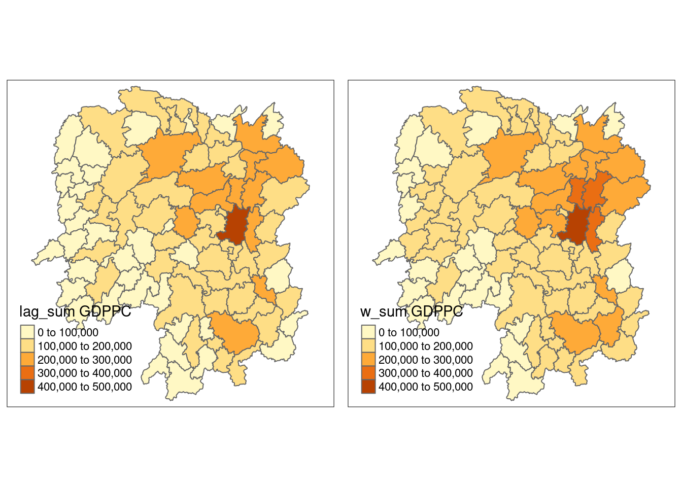
Which method to use?
Spatial Lag with Row-Standardized Weights
Use this method when you want each point to have an equal influence across all of its neighbors, regardless of the number of neighbors it has.
It is most appropriate when you expect the spatial relationships to be similar across your dataset (i.e., you don’t want points with many neighbors to overwhelm points with fewer neighbors).
Commonly used in spatial autoregressive models (SAR) like the spatial lag model (SLM).
Typically used in spatial econometrics when you’re interested in modeling the spillover effects or dependence of a variable across space.
Example: In a housing price study, you might use this if you want to see how the prices of neighboring houses (standardized by distance) affect the price of a given house.
Spatial Lag as a Sum of Neighboring Values
Use this method when you want to model the total influence of the neighbors without diluting the effect based on the number of neighbors.
It is useful when the total volume or intensity of the neighboring values matters, rather than their average or relative influence.
Best for situations where cumulative effects are important, like when you’re interested in understanding the total influence of surrounding areas (e.g., total population or pollution).
This method might be relevant in studies where absolute values are important, such as environmental studies focusing on total pollution from neighboring regions.
Example: In studying air pollution, you might want the sum of pollution from all neighboring areas rather than an average influence, since the total pollution matters.
Spatial Window Average
Use this method when you want to calculate a local average around each point within a specific window size (e.g., all points within a 10 km radius).
It is useful when you want to smooth the data or when you’re focusing on local averages rather than global or cumulative effects.
This is often used in spatial smoothing or when looking for local trends in spatial data.
In epidemiology, if you’re studying the average infection rate within a region (based on nearby regions), you might use a spatial window average to model localized clusters of infection.
Spatial Window Sum
Use this method when the total quantity or accumulation of a variable in a region is important, and you want to sum the values within a certain distance from each point.
It’s useful for applications where the cumulative total of a variable within a region matters more than its average.
This method is often used in environmental studies, resource management, or studies where total values in a region (like total population or total resource availability) are critical.
Example: In disaster management, if you’re estimating the total population within a flood-prone zone, you’d use a spatial window sum to calculate how many people live within the danger area.
Use each method depending on whether you care about relative influence, total influence, local average, or total value.