pacman::p_load(sf, raster, spatstat, tmap, tidyverse)Hands-on Exercise 3
1st Order Spatial Point Patterns Analysis Methods
Spatial Point Pattern Analysis (SPPA) is a method used to evaluate the pattern or distribution of a set of points on a surface. To begin with, we need to gather data on the locations of these childcare centres and their corresponding coordinates. We can use geographic information systems (GIS) software to do this. Once we have this data, we can then analyze it using SPPA. The first step is to identify the spatial point processes that exist within a given area.
After identifying these patterns, we can determine whether there are any locations with higher concentrations of childcare centres. This information can be used to gain insights into possible trends or patterns in the distribution of these centres, and help policy makers make informed decisions about where new centres should be located.
Installing and loading R packages
In this hands-on exercise, five R packages will be used, they are:
sf, a relatively new R package specially designed to import, manage and process vector-based geospatial data in R.
spatstat, which has a wide range of useful functions for point pattern analysis. In this hands-on exercise, it will be used to perform 1st- and 2nd-order spatial point patterns analysis and derive kernel density estimation (KDE) layer.
raster which reads, writes, manipulates, analyses and model of gridded spatial data (i.e. raster). In this hands-on exercise, it will be used to convert image output generate by spatstat into raster format.
maptools which provides a set of tools for manipulating geographic data. In this hands-on exercise, we mainly use it to convert Spatial objects into ppp format of spatstat.
tmap which provides functions for plotting cartographic quality static point patterns maps or interactive maps by using leaflet API.
childcare_sf <- st_read("data/child-care-services-geojson.geojson") %>%
  st_transform(crs = 3414)
Reading layer `child-care-services-geojson' from data source
`/home/tropicbliss/GitHub/quarto-project/Hands-on_Ex/Hands-on_Ex03/data/child-care-services-geojson.geojson'
using driver `GeoJSON'
Simple feature collection with 1545 features and 2 fields
Geometry type: POINT
Dimension: XYZ
Bounding box: xmin: 103.6824 ymin: 1.248403 xmax: 103.9897 ymax: 1.462134
z_range: zmin: 0 zmax: 0
Geodetic CRS: WGS 84sg_sf <- st_read(dsn = "data", layer="CostalOutline")Reading layer `CostalOutline' from data source
`/home/tropicbliss/GitHub/quarto-project/Hands-on_Ex/Hands-on_Ex03/data'
using driver `ESRI Shapefile'
Simple feature collection with 60 features and 4 fields
Geometry type: POLYGON
Dimension: XY
Bounding box: xmin: 2663.926 ymin: 16357.98 xmax: 56047.79 ymax: 50244.03
Projected CRS: SVY21In this case, CostalOutline is the name of the Shapefile.
mpsz_sf <- st_read(dsn = "data", layer = "MP14_SUBZONE_WEB_PL")Reading layer `MP14_SUBZONE_WEB_PL' from data source
`/home/tropicbliss/GitHub/quarto-project/Hands-on_Ex/Hands-on_Ex03/data'
using driver `ESRI Shapefile'
Simple feature collection with 323 features and 15 fields
Geometry type: MULTIPOLYGON
Dimension: XY
Bounding box: xmin: 2667.538 ymin: 15748.72 xmax: 56396.44 ymax: 50256.33
Projected CRS: SVY21st_crs(sg_sf)Coordinate Reference System:
User input: SVY21
wkt:
PROJCRS["SVY21",
BASEGEOGCRS["SVY21[WGS84]",
DATUM["World Geodetic System 1984",
ELLIPSOID["WGS 84",6378137,298.257223563,
LENGTHUNIT["metre",1]],
ID["EPSG",6326]],
PRIMEM["Greenwich",0,
ANGLEUNIT["Degree",0.0174532925199433]]],
CONVERSION["unnamed",
METHOD["Transverse Mercator",
ID["EPSG",9807]],
PARAMETER["Latitude of natural origin",1.36666666666667,
ANGLEUNIT["Degree",0.0174532925199433],
ID["EPSG",8801]],
PARAMETER["Longitude of natural origin",103.833333333333,
ANGLEUNIT["Degree",0.0174532925199433],
ID["EPSG",8802]],
PARAMETER["Scale factor at natural origin",1,
SCALEUNIT["unity",1],
ID["EPSG",8805]],
PARAMETER["False easting",28001.642,
LENGTHUNIT["metre",1],
ID["EPSG",8806]],
PARAMETER["False northing",38744.572,
LENGTHUNIT["metre",1],
ID["EPSG",8807]]],
CS[Cartesian,2],
AXIS["(E)",east,
ORDER[1],
LENGTHUNIT["metre",1,
ID["EPSG",9001]]],
AXIS["(N)",north,
ORDER[2],
LENGTHUNIT["metre",1,
ID["EPSG",9001]]]]st_crs(mpsz_sf)Coordinate Reference System:
User input: SVY21
wkt:
PROJCRS["SVY21",
BASEGEOGCRS["SVY21[WGS84]",
DATUM["World Geodetic System 1984",
ELLIPSOID["WGS 84",6378137,298.257223563,
LENGTHUNIT["metre",1]],
ID["EPSG",6326]],
PRIMEM["Greenwich",0,
ANGLEUNIT["Degree",0.0174532925199433]]],
CONVERSION["unnamed",
METHOD["Transverse Mercator",
ID["EPSG",9807]],
PARAMETER["Latitude of natural origin",1.36666666666667,
ANGLEUNIT["Degree",0.0174532925199433],
ID["EPSG",8801]],
PARAMETER["Longitude of natural origin",103.833333333333,
ANGLEUNIT["Degree",0.0174532925199433],
ID["EPSG",8802]],
PARAMETER["Scale factor at natural origin",1,
SCALEUNIT["unity",1],
ID["EPSG",8805]],
PARAMETER["False easting",28001.642,
LENGTHUNIT["metre",1],
ID["EPSG",8806]],
PARAMETER["False northing",38744.572,
LENGTHUNIT["metre",1],
ID["EPSG",8807]]],
CS[Cartesian,2],
AXIS["(E)",east,
ORDER[1],
LENGTHUNIT["metre",1,
ID["EPSG",9001]]],
AXIS["(N)",north,
ORDER[2],
LENGTHUNIT["metre",1,
ID["EPSG",9001]]]]It seems like the projected CRS are all in order (SVY21).
Mapping the geospatial data sets
tmap_mode('plot')tmap mode set to plottingtm_shape(mpsz_sf) +
tm_fill() + # draw polygons without borders
tm_borders() + # draw borders
tm_shape(childcare_sf) +
tm_dots() # draw points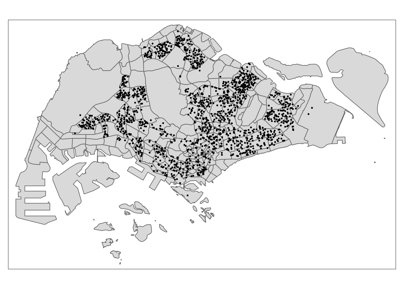
You can also create a pin map using the Leaflet API:
tmap_mode('view')tmap mode set to interactive viewingtm_shape(childcare_sf) +
tm_dots()The advantage of this interactive pin map is it allows us to navigate and zoom around the map freely. We can also query the information of each simple feature (i.e. the point) by clicking of them. Last but not least, you can also change the background of the internet map layer. Currently, three internet map layers are provided. They are: ESRI.WorldGrayCanvas, OpenStreetMap, and ESRI.WorldTopoMap. The default is ESRI.WorldGrayCanvas.
Always remember to switch back to plot mode after the interactive map. This is because, each interactive mode will consume a connection. You should also avoid displaying ecessive numbers of interactive maps (i.e. not more than 10) in one RMarkdown document when publish on Netlify.
tmap_mode("plot")tmap mode set to plottingWhile simple features is popular, many geospatial packages still require sp’s Spatial class. Here is how we convert them back to Spatial:
childcare <- as_Spatial(childcare_sf)
mpsz <- as_Spatial(mpsz_sf)
sg <- as_Spatial(sg_sf)summary(childcare)Object of class SpatialPointsDataFrame
Coordinates:
min max
coords.x1 11203.01 45404.24
coords.x2 25667.60 49300.88
coords.x3 0.00 0.00
Is projected: TRUE
proj4string :
[+proj=tmerc +lat_0=1.36666666666667 +lon_0=103.833333333333 +k=1
+x_0=28001.642 +y_0=38744.572 +ellps=WGS84 +towgs84=0,0,0,0,0,0,0
+units=m +no_defs]
Number of points: 1545
Data attributes:
Name Description
Length:1545 Length:1545
Class :character Class :character
Mode :character Mode :character summary(mpsz)Object of class SpatialPolygonsDataFrame
Coordinates:
min max
x 2667.538 56396.44
y 15748.721 50256.33
Is projected: TRUE
proj4string :
[+proj=tmerc +lat_0=1.36666666666667 +lon_0=103.833333333333 +k=1
+x_0=28001.642 +y_0=38744.572 +datum=WGS84 +units=m +no_defs]
Data attributes:
OBJECTID SUBZONE_NO SUBZONE_N SUBZONE_C
Min. : 1.0 Min. : 1.000 Length:323 Length:323
1st Qu.: 81.5 1st Qu.: 2.000 Class :character Class :character
Median :162.0 Median : 4.000 Mode :character Mode :character
Mean :162.0 Mean : 4.625
3rd Qu.:242.5 3rd Qu.: 6.500
Max. :323.0 Max. :17.000
CA_IND PLN_AREA_N PLN_AREA_C REGION_N
Length:323 Length:323 Length:323 Length:323
Class :character Class :character Class :character Class :character
Mode :character Mode :character Mode :character Mode :character
REGION_C INC_CRC FMEL_UPD_D X_ADDR
Length:323 Length:323 Min. :2014-12-05 Min. : 5093
Class :character Class :character 1st Qu.:2014-12-05 1st Qu.:21864
Mode :character Mode :character Median :2014-12-05 Median :28465
Mean :2014-12-05 Mean :27257
3rd Qu.:2014-12-05 3rd Qu.:31674
Max. :2014-12-05 Max. :50425
Y_ADDR SHAPE_Leng SHAPE_Area
Min. :19579 Min. : 871.5 Min. : 39438
1st Qu.:31776 1st Qu.: 3709.6 1st Qu.: 628261
Median :35113 Median : 5211.9 Median : 1229894
Mean :36106 Mean : 6524.4 Mean : 2420882
3rd Qu.:39869 3rd Qu.: 6942.6 3rd Qu.: 2106483
Max. :49553 Max. :68083.9 Max. :69748299 summary(sg)Object of class SpatialPolygonsDataFrame
Coordinates:
min max
x 2663.926 56047.79
y 16357.981 50244.03
Is projected: TRUE
proj4string :
[+proj=tmerc +lat_0=1.36666666666667 +lon_0=103.833333333333 +k=1
+x_0=28001.642 +y_0=38744.572 +datum=WGS84 +units=m +no_defs]
Data attributes:
GDO_GID MSLINK MAPID COSTAL_NAM
Min. : 1.00 Min. : 1.00 Min. :0 Length:60
1st Qu.:15.75 1st Qu.:17.75 1st Qu.:0 Class :character
Median :30.50 Median :33.50 Median :0 Mode :character
Mean :30.50 Mean :33.77 Mean :0
3rd Qu.:45.25 3rd Qu.:49.25 3rd Qu.:0
Max. :60.00 Max. :67.00 Max. :0 spatstat requires the analytical data in ppp object form. There is no direct way to convert a Spatial* classes into ppp object. We need to convert the Spatial classes* into Spatial object first.
What is ppp object form?
A ppp object is a type of data structure used in the spatstat package in R for handling spatial point pattern data. The ppp stands for “planar point pattern,” and it represents a collection of points that are typically used in the analysis of spatial point processes.
Points
The ppp object contains the coordinates of the points in the point pattern. These are stored as two numeric vectors, x and y, which represent the Cartesian coordinates of the points.
Window
This component defines the observation window, i.e., the area in which the points are observed. The window can be a simple rectangle or a more complex polygonal region. The window is typically an object of class owin, which specifies the boundaries within which the points are contained.
Marks
The ppp object can include additional data associated with each point, known as “marks.” Marks can be any type of data, such as categorical labels, numerical values, or even more complex data structures. Marks add a second level of information to the point pattern, allowing for marked point process analysis.
Converting to ppp
First, we have to convert the sf Spatial classes into generic sp objects.
childcare_sp <- as(childcare, "SpatialPoints")
sg_sp <- as(sg, "SpatialPolygons")summary(childcare_sp)Object of class SpatialPoints
Coordinates:
min max
coords.x1 11203.01 45404.24
coords.x2 25667.60 49300.88
coords.x3 0.00 0.00
Is projected: TRUE
proj4string :
[+proj=tmerc +lat_0=1.36666666666667 +lon_0=103.833333333333 +k=1
+x_0=28001.642 +y_0=38744.572 +ellps=WGS84 +towgs84=0,0,0,0,0,0,0
+units=m +no_defs]
Number of points: 1545summary(sg_sp)Object of class SpatialPolygons
Coordinates:
min max
x 2663.926 56047.79
y 16357.981 50244.03
Is projected: TRUE
proj4string :
[+proj=tmerc +lat_0=1.36666666666667 +lon_0=103.833333333333 +k=1
+x_0=28001.642 +y_0=38744.572 +datum=WGS84 +units=m +no_defs]Next, we need to convert the generic sp objects into spatstat’s ppp object.
childcare_ppp <- as.ppp(childcare_sf)Warning in as.ppp.sf(childcare_sf): only first attribute column is used for
markschildcare_pppMarked planar point pattern: 1545 points
marks are of storage type 'character'
window: rectangle = [11203.01, 45404.24] x [25667.6, 49300.88] unitsNow, let’s plot childcare_ppp:
plot(childcare_ppp)Warning in default.charmap(ntypes, chars): Too many types to display every type
as a different characterWarning: Only 10 out of 1545 symbols are shown in the symbol map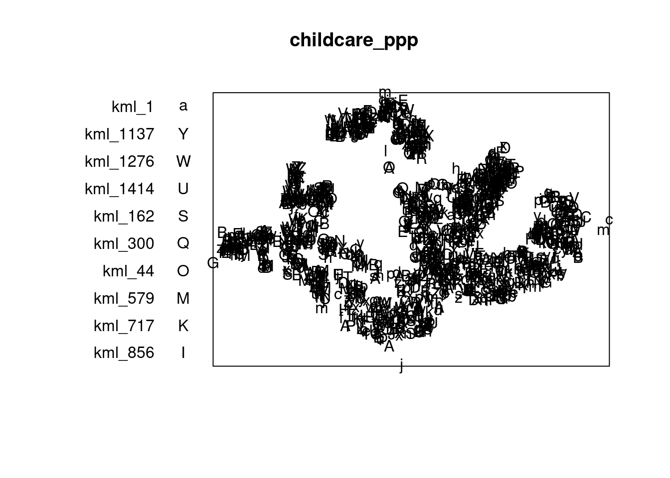
summary(childcare_ppp)Marked planar point pattern: 1545 points
Average intensity 1.91145e-06 points per square unit
Coordinates are given to 11 decimal places
marks are of type 'character'
Summary:
Length Class Mode
1545 character character
Window: rectangle = [11203.01, 45404.24] x [25667.6, 49300.88] units
(34200 x 23630 units)
Window area = 808287000 square unitsIn spatial point pattern analysis, the concept of duplicates or coincident points refers to multiple points that occupy the exact same location in space.
Many statistical methods in spatial point pattern analysis are based on the assumption that the underlying point process is simple. A simple point process means that no two points in the process can occupy the exact same location (i.e., they cannot be coincident).
If points are coincident, this assumption is violated, and the statistical methods that rely on this assumption may produce invalid or misleading results.
Thus, let’s check if there are any duplicate points:
any(duplicated(childcare_ppp))[1] FALSEAs you can see, there doesn’t seem to be any duplicated data point.
To count the number of co-indicence point, we will use the multiplicity() function as shown in the code chunk below.
multiplicity(childcare_ppp) [1] 1 1 1 1 1 1 1 1 1 1 1 1 1 1 1 1 1 1 1 1 1 1 1 1 1 1 1 1 1 1 1 1 1 1 1 1 1
[38] 1 1 1 1 1 1 1 1 1 1 1 1 1 1 1 1 1 1 1 1 1 1 1 1 1 1 1 1 1 1 1 1 1 1 1 1 1
[75] 1 1 1 1 1 1 1 1 1 1 1 1 1 1 1 1 1 1 1 1 1 1 1 1 1 1 1 1 1 1 1 1 1 1 1 1 1
[112] 1 1 1 1 1 1 1 1 1 1 1 1 1 1 1 1 1 1 1 1 1 1 1 1 1 1 1 1 1 1 1 1 1 1 1 1 1
[149] 1 1 1 1 1 1 1 1 1 1 1 1 1 1 1 1 1 1 1 1 1 1 1 1 1 1 1 1 1 1 1 1 1 1 1 1 1
[186] 1 1 1 1 1 1 1 1 1 1 1 1 1 1 1 1 1 1 1 1 1 1 1 1 1 1 1 1 1 1 1 1 1 1 1 1 1
[223] 1 1 1 1 1 1 1 1 1 1 1 1 1 1 1 1 1 1 1 1 1 1 1 1 1 1 1 1 1 1 1 1 1 1 1 1 1
[260] 1 1 1 1 1 1 1 1 1 1 1 1 1 1 1 1 1 1 1 1 1 1 1 1 1 1 1 1 1 1 1 1 1 1 1 1 1
[297] 1 1 1 1 1 1 1 1 1 1 1 1 1 1 1 1 1 1 1 1 1 1 1 1 1 1 1 1 1 1 1 1 1 1 1 1 1
[334] 1 1 1 1 1 1 1 1 1 1 1 1 1 1 1 1 1 1 1 1 1 1 1 1 1 1 1 1 1 1 1 1 1 1 1 1 1
[371] 1 1 1 1 1 1 1 1 1 1 1 1 1 1 1 1 1 1 1 1 1 1 1 1 1 1 1 1 1 1 1 1 1 1 1 1 1
[408] 1 1 1 1 1 1 1 1 1 1 1 1 1 1 1 1 1 1 1 1 1 1 1 1 1 1 1 1 1 1 1 1 1 1 1 1 1
[445] 1 1 1 1 1 1 1 1 1 1 1 1 1 1 1 1 1 1 1 1 1 1 1 1 1 1 1 1 1 1 1 1 1 1 1 1 1
[482] 1 1 1 1 1 1 1 1 1 1 1 1 1 1 1 1 1 1 1 1 1 1 1 1 1 1 1 1 1 1 1 1 1 1 1 1 1
[519] 1 1 1 1 1 1 1 1 1 1 1 1 1 1 1 1 1 1 1 1 1 1 1 1 1 1 1 1 1 1 1 1 1 1 1 1 1
[556] 1 1 1 1 1 1 1 1 1 1 1 1 1 1 1 1 1 1 1 1 1 1 1 1 1 1 1 1 1 1 1 1 1 1 1 1 1
[593] 1 1 1 1 1 1 1 1 1 1 1 1 1 1 1 1 1 1 1 1 1 1 1 1 1 1 1 1 1 1 1 1 1 1 1 1 1
[630] 1 1 1 1 1 1 1 1 1 1 1 1 1 1 1 1 1 1 1 1 1 1 1 1 1 1 1 1 1 1 1 1 1 1 1 1 1
[667] 1 1 1 1 1 1 1 1 1 1 1 1 1 1 1 1 1 1 1 1 1 1 1 1 1 1 1 1 1 1 1 1 1 1 1 1 1
[704] 1 1 1 1 1 1 1 1 1 1 1 1 1 1 1 1 1 1 1 1 1 1 1 1 1 1 1 1 1 1 1 1 1 1 1 1 1
[741] 1 1 1 1 1 1 1 1 1 1 1 1 1 1 1 1 1 1 1 1 1 1 1 1 1 1 1 1 1 1 1 1 1 1 1 1 1
[778] 1 1 1 1 1 1 1 1 1 1 1 1 1 1 1 1 1 1 1 1 1 1 1 1 1 1 1 1 1 1 1 1 1 1 1 1 1
[815] 1 1 1 1 1 1 1 1 1 1 1 1 1 1 1 1 1 1 1 1 1 1 1 1 1 1 1 1 1 1 1 1 1 1 1 1 1
[852] 1 1 1 1 1 1 1 1 1 1 1 1 1 1 1 1 1 1 1 1 1 1 1 1 1 1 1 1 1 1 1 1 1 1 1 1 1
[889] 1 1 1 1 1 1 1 1 1 1 1 1 1 1 1 1 1 1 1 1 1 1 1 1 1 1 1 1 1 1 1 1 1 1 1 1 1
[926] 1 1 1 1 1 1 1 1 1 1 1 1 1 1 1 1 1 1 1 1 1 1 1 1 1 1 1 1 1 1 1 1 1 1 1 1 1
[963] 1 1 1 1 1 1 1 1 1 1 1 1 1 1 1 1 1 1 1 1 1 1 1 1 1 1 1 1 1 1 1 1 1 1 1 1 1
[1000] 1 1 1 1 1 1 1 1 1 1 1 1 1 1 1 1 1 1 1 1 1 1 1 1 1 1 1 1 1 1 1 1 1 1 1 1 1
[1037] 1 1 1 1 1 1 1 1 1 1 1 1 1 1 1 1 1 1 1 1 1 1 1 1 1 1 1 1 1 1 1 1 1 1 1 1 1
[1074] 1 1 1 1 1 1 1 1 1 1 1 1 1 1 1 1 1 1 1 1 1 1 1 1 1 1 1 1 1 1 1 1 1 1 1 1 1
[1111] 1 1 1 1 1 1 1 1 1 1 1 1 1 1 1 1 1 1 1 1 1 1 1 1 1 1 1 1 1 1 1 1 1 1 1 1 1
[1148] 1 1 1 1 1 1 1 1 1 1 1 1 1 1 1 1 1 1 1 1 1 1 1 1 1 1 1 1 1 1 1 1 1 1 1 1 1
[1185] 1 1 1 1 1 1 1 1 1 1 1 1 1 1 1 1 1 1 1 1 1 1 1 1 1 1 1 1 1 1 1 1 1 1 1 1 1
[1222] 1 1 1 1 1 1 1 1 1 1 1 1 1 1 1 1 1 1 1 1 1 1 1 1 1 1 1 1 1 1 1 1 1 1 1 1 1
[1259] 1 1 1 1 1 1 1 1 1 1 1 1 1 1 1 1 1 1 1 1 1 1 1 1 1 1 1 1 1 1 1 1 1 1 1 1 1
[1296] 1 1 1 1 1 1 1 1 1 1 1 1 1 1 1 1 1 1 1 1 1 1 1 1 1 1 1 1 1 1 1 1 1 1 1 1 1
[1333] 1 1 1 1 1 1 1 1 1 1 1 1 1 1 1 1 1 1 1 1 1 1 1 1 1 1 1 1 1 1 1 1 1 1 1 1 1
[1370] 1 1 1 1 1 1 1 1 1 1 1 1 1 1 1 1 1 1 1 1 1 1 1 1 1 1 1 1 1 1 1 1 1 1 1 1 1
[1407] 1 1 1 1 1 1 1 1 1 1 1 1 1 1 1 1 1 1 1 1 1 1 1 1 1 1 1 1 1 1 1 1 1 1 1 1 1
[1444] 1 1 1 1 1 1 1 1 1 1 1 1 1 1 1 1 1 1 1 1 1 1 1 1 1 1 1 1 1 1 1 1 1 1 1 1 1
[1481] 1 1 1 1 1 1 1 1 1 1 1 1 1 1 1 1 1 1 1 1 1 1 1 1 1 1 1 1 1 1 1 1 1 1 1 1 1
[1518] 1 1 1 1 1 1 1 1 1 1 1 1 1 1 1 1 1 1 1 1 1 1 1 1 1 1 1 1If we want to know how many locations have more than one point event, we can use the code chunk below:
sum(multiplicity(childcare_ppp) > 1)[1] 0To view the locations of any duplicate point events, we will plot childcare data by using the code chunk below:
coincident_points <- childcare_sf[duplicated(st_geometry(childcare_sf)), ]
tmap_mode('view')
tmap mode set to interactive viewingtm_shape(coincident_points) +
tm_dots(alpha=0.4,
size=0.05)tmap_mode("plot")tmap mode set to plottingThere are three ways to overcome this problem. The easiest way is to delete the duplicates. But, that will also mean that some useful point events will be lost.
The second solution is use jittering. It is used to add a small amount of random noise to the coordinates of points in a spatial point pattern. This process, often referred to as “jittering,” helps to separate coincident points (points that have the exact same coordinates) by moving them slightly apart. This can be particularly useful in spatial analyses where coincident points might violate assumptions, such as the assumption that points are not exactly coincident.
The third solution is to make each point “unique” and then attach the duplicates of the points to the patterns as marks, as attributes of the points. Then you would need analytical techniques that take into account these marks.
The code chunk below implements the jittering approach.
childcare_ppp_jit <- rjitter(childcare_ppp,
                             retry=TRUE,
                             nsim=1,
                             drop=TRUE)
Let’s see if there are any duplicates now:
any(duplicated(childcare_ppp_jit))[1] FALSECreating owin object
When analysing spatial point patterns, it is a good practice to confine the analysis with a geographical area like Singapore boundary. In spatstat, an object called owin is specially designed to represent this polygonal region.
The code chunk below is used to covert sg SpatialPolygon object into owin object of spatstat.
sg_owin <- as.owin(sg_sf)The ouput object can be displayed by using plot() function
plot(sg_owin)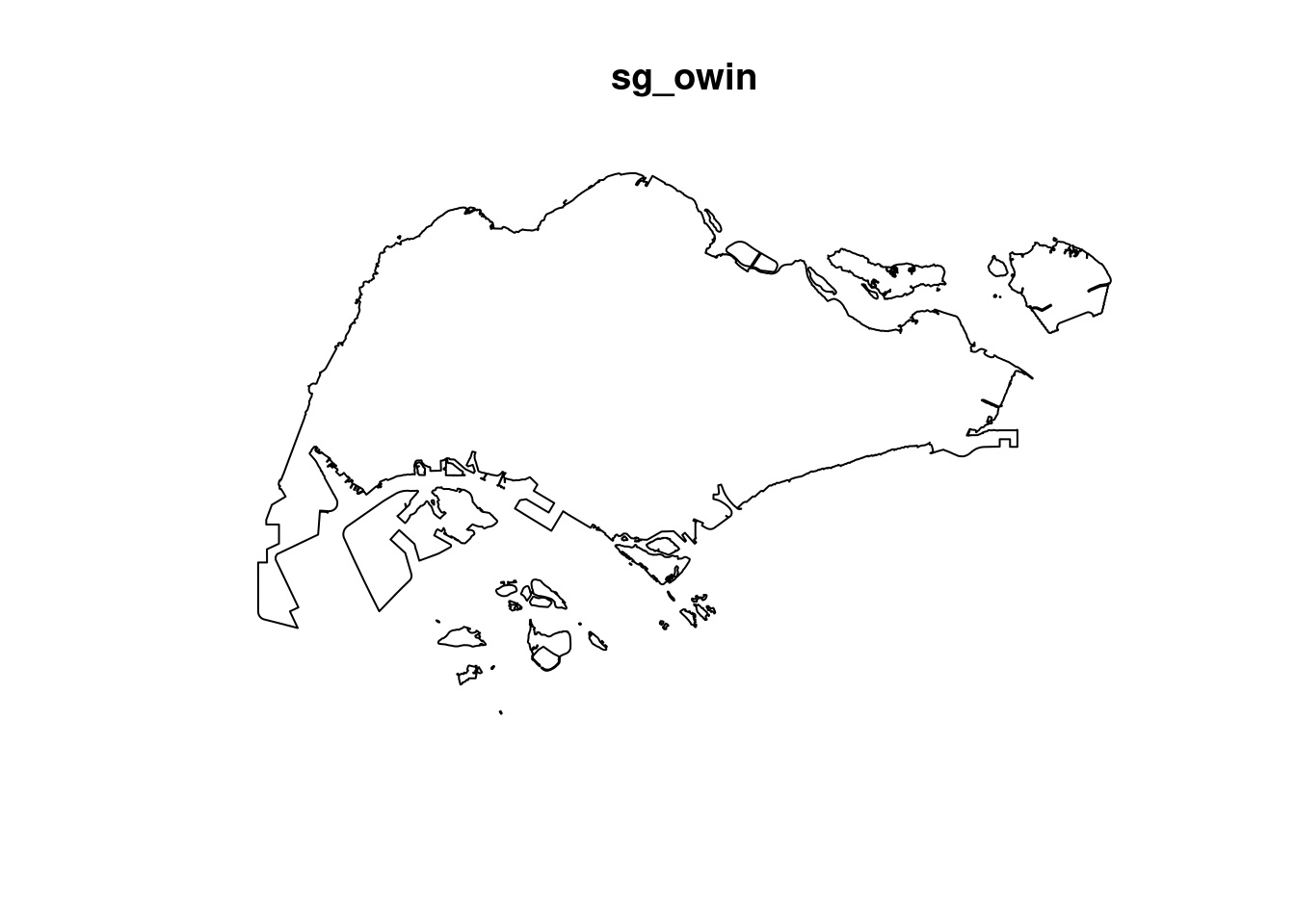
summary(sg_owin)Window: polygonal boundary
50 separate polygons (1 hole)
vertices area relative.area
polygon 1 (hole) 30 -7081.18 -9.76e-06
polygon 2 55 82537.90 1.14e-04
polygon 3 90 415092.00 5.72e-04
polygon 4 49 16698.60 2.30e-05
polygon 5 38 24249.20 3.34e-05
polygon 6 976 23344700.00 3.22e-02
polygon 7 721 1927950.00 2.66e-03
polygon 8 1992 9992170.00 1.38e-02
polygon 9 330 1118960.00 1.54e-03
polygon 10 175 925904.00 1.28e-03
polygon 11 115 928394.00 1.28e-03
polygon 12 24 6352.39 8.76e-06
polygon 13 190 202489.00 2.79e-04
polygon 14 37 10170.50 1.40e-05
polygon 15 25 16622.70 2.29e-05
polygon 16 10 2145.07 2.96e-06
polygon 17 66 16184.10 2.23e-05
polygon 18 5195 636837000.00 8.78e-01
polygon 19 76 312332.00 4.31e-04
polygon 20 627 31891300.00 4.40e-02
polygon 21 20 32842.00 4.53e-05
polygon 22 42 55831.70 7.70e-05
polygon 23 67 1313540.00 1.81e-03
polygon 24 734 4690930.00 6.47e-03
polygon 25 16 3194.60 4.40e-06
polygon 26 15 4872.96 6.72e-06
polygon 27 15 4464.20 6.15e-06
polygon 28 14 5466.74 7.54e-06
polygon 29 37 5261.94 7.25e-06
polygon 30 111 662927.00 9.14e-04
polygon 31 69 56313.40 7.76e-05
polygon 32 143 145139.00 2.00e-04
polygon 33 397 2488210.00 3.43e-03
polygon 34 90 115991.00 1.60e-04
polygon 35 98 62682.90 8.64e-05
polygon 36 165 338736.00 4.67e-04
polygon 37 130 94046.50 1.30e-04
polygon 38 93 430642.00 5.94e-04
polygon 39 16 2010.46 2.77e-06
polygon 40 415 3253840.00 4.49e-03
polygon 41 30 10838.20 1.49e-05
polygon 42 53 34400.30 4.74e-05
polygon 43 26 8347.58 1.15e-05
polygon 44 74 58223.40 8.03e-05
polygon 45 327 2169210.00 2.99e-03
polygon 46 177 467446.00 6.44e-04
polygon 47 46 699702.00 9.65e-04
polygon 48 6 16841.00 2.32e-05
polygon 49 13 70087.30 9.66e-05
polygon 50 4 9459.63 1.30e-05
enclosing rectangle: [2663.93, 56047.79] x [16357.98, 50244.03] units
(53380 x 33890 units)
Window area = 725376000 square units
Fraction of frame area: 0.401Combining point events object and owin object
In this last step of geospatial data wrangling, we will extract childcare events that are located within Singapore by using the code chunk below.
childcareSG_ppp = childcare_ppp[sg_owin]
summary(childcareSG_ppp)Marked planar point pattern: 1545 points
Average intensity 2.129929e-06 points per square unit
Coordinates are given to 11 decimal places
marks are of type 'character'
Summary:
Length Class Mode
1545 character character
Window: polygonal boundary
50 separate polygons (1 hole)
                 vertices         area relative.area
polygon 1 (hole)       30     -7081.18     -9.76e-06
polygon 2              55     82537.90      1.14e-04
polygon 3              90    415092.00      5.72e-04
polygon 4              49     16698.60      2.30e-05
polygon 5              38     24249.20      3.34e-05
polygon 6             976  23344700.00      3.22e-02
polygon 7             721   1927950.00      2.66e-03
polygon 8            1992   9992170.00      1.38e-02
polygon 9             330   1118960.00      1.54e-03
polygon 10            175    925904.00      1.28e-03
polygon 11            115    928394.00      1.28e-03
polygon 12             24      6352.39      8.76e-06
polygon 13            190    202489.00      2.79e-04
polygon 14             37     10170.50      1.40e-05
polygon 15             25     16622.70      2.29e-05
polygon 16             10      2145.07      2.96e-06
polygon 17             66     16184.10      2.23e-05
polygon 18           5195 636837000.00      8.78e-01
polygon 19             76    312332.00      4.31e-04
polygon 20            627  31891300.00      4.40e-02
polygon 21             20     32842.00      4.53e-05
polygon 22             42     55831.70      7.70e-05
polygon 23             67   1313540.00      1.81e-03
polygon 24            734   4690930.00      6.47e-03
polygon 25             16      3194.60      4.40e-06
polygon 26             15      4872.96      6.72e-06
polygon 27             15      4464.20      6.15e-06
polygon 28             14      5466.74      7.54e-06
polygon 29             37      5261.94      7.25e-06
polygon 30            111    662927.00      9.14e-04
polygon 31             69     56313.40      7.76e-05
polygon 32            143    145139.00      2.00e-04
polygon 33            397   2488210.00      3.43e-03
polygon 34             90    115991.00      1.60e-04
polygon 35             98     62682.90      8.64e-05
polygon 36            165    338736.00      4.67e-04
polygon 37            130     94046.50      1.30e-04
polygon 38             93    430642.00      5.94e-04
polygon 39             16      2010.46      2.77e-06
polygon 40            415   3253840.00      4.49e-03
polygon 41             30     10838.20      1.49e-05
polygon 42             53     34400.30      4.74e-05
polygon 43             26      8347.58      1.15e-05
polygon 44             74     58223.40      8.03e-05
polygon 45            327   2169210.00      2.99e-03
polygon 46            177    467446.00      6.44e-04
polygon 47             46    699702.00      9.65e-04
polygon 48              6     16841.00      2.32e-05
polygon 49             13     70087.30      9.66e-05
polygon 50              4      9459.63      1.30e-05
enclosing rectangle: [2663.93, 56047.79] x [16357.98, 50244.03] units
                     (53380 x 33890 units)
Window area = 725376000 square units
Fraction of frame area: 0.401plot(childcareSG_ppp)Warning in default.charmap(ntypes, chars): Too many types to display every type
as a different characterWarning: Only 10 out of 1545 symbols are shown in the symbol map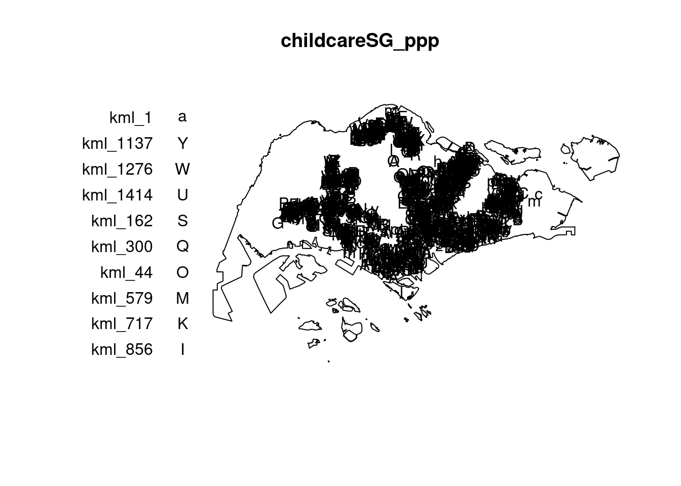
First-order Spatial Point Patterns Analysis
In this section, you will learn how to perform first-order SPPA by using spatstat package. The hands-on exercise will focus on:
deriving kernel density estimation (KDE) layer for visualising and exploring the intensity of point processes,
performing Confirmatory Spatial Point Patterns Analysis by using Nearest Neighbour statistics.
Kernel Density Estimation
Kernel Density Estimation (KDE) is a non-parametric method (does not assume any specific underlying distribution for the data) used to estimate the probability density function (PDF) of a random variable based on a finite sample of data points. In spatial analysis, KDE is often used to estimate the intensity or density of events (such as crime incidents, animal sightings, or disease cases) across a geographical area.
Clustered (groups of POI close together)
Random (spread out but with irregular spacing)
Uniform (spread out but have regular spacing)
Mapping stuff out is exploratory. To quantify it we can employ hypothesis testing.
We essentially count the number of points of interest in a particular area (which we can specify) and calculate the density (or intensity).
In this section, you will learn how to compute the kernel density estimation (KDE) of childcare services in Singapore.
Automatic bandwidth selection method
Note: Even though it is called “automatic bandwidth”, they are considered fixed bandwidth methods (you calculate density with the same area throughout). Use adaptive bandwidth instead if you have highly skewed data. Use fixed bandwidth if you are comparing KDE between regions.x`
The code chunk below computes a kernel density by using the following configurations of density() of spatstat:
bw.diggle() automatic bandwidth selection method. Other recommended methods are bw.CvL(), bw.scott() or bw.ppl().
The smoothing kernel used is gaussian, which is the default. Other smoothing methods are: “epanechnikov”, “quartic” or “disc”.
The
edgeparameter controls whether edge correction should be applied. Edge correction accounts for the fact that points near the boundaries of the observation window have fewer neighbors and, without correction, could lead to underestimation of density near the edges.Setting
edge = TRUEensures that edge correction is applied, which adjusts the density estimate near the borders to compensate for this bias.- The intensity estimate is corrected for edge effect bias by using method described by Jones (1993) and Diggle (2010, equation 18.9). The default is FALSE.
kde_childcareSG_bw <- density(childcareSG_ppp,
                              sigma=bw.diggle,
                              edge=TRUE,
                            kernel="gaussian")
The plot() function of Base R is then used to display the kernel density derived.
plot(kde_childcareSG_bw)
The density values of the output range from 0 to 0.000035 which is way too small to comprehend. This is because the default unit of measurement of svy21 is in meter. As a result, the density values computed is in “number of points per square meter”.
Before we move on to next section, it is good to know that you can retrieve the bandwidth used to compute the kde layer by using the code chunk below.
bw <- bw.diggle(childcareSG_ppp)
bw
sigma
298.4095 The bandwidth in the context of Kernel Density Estimation (KDE) is a critical parameter that determines the level of smoothing applied to the data when estimating the density. It controls how much each data point influences the estimate of the density around it.
To convert the unit of measurement from meter to kilometer:
childcareSG_ppp.km <- rescale.ppp(childcareSG_ppp, 1000, "km")Now, we can re-run density() using the resale data set and plot the output KDE map.
kde_childcareSG.bw <- density(childcareSG_ppp.km, sigma=bw.diggle, edge=TRUE, kernel="gaussian")
plot(kde_childcareSG.bw)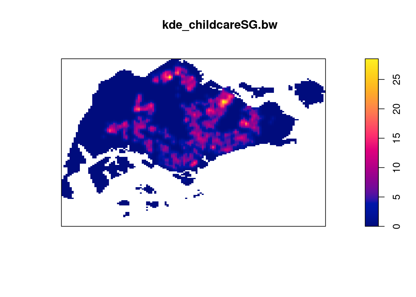
Working with different bandwidth methods
bw.CvL(childcareSG_ppp.km) sigma
4.543278 bw.scott(childcareSG_ppp.km) sigma.x sigma.y
2.224898 1.450966 bw.ppl(childcareSG_ppp.km) sigma
0.3897114 bw.diggle(childcareSG_ppp.km) sigma
0.2984095 Baddeley et. (2016) suggested the use of the bw.ppl() algorithm because in their experience it tends to produce the more appropriate values when the pattern consists predominantly of tight clusters. But they also insist that if the purpose of once study is to detect a single tight cluster in the midst of random noise then the bw.diggle() method seems to work best.
The code chunk below will be used to compare the output of using bw.diggle and bw.ppl methods:
kde_childcareSG.ppl <- density(childcareSG_ppp.km,
                               sigma=bw.ppl,
                               edge=TRUE,
                               kernel="gaussian")
par(mfrow=c(1,2))
plot(kde_childcareSG.bw, main = "bw.diggle")
plot(kde_childcareSG.ppl, main = "bw.ppl")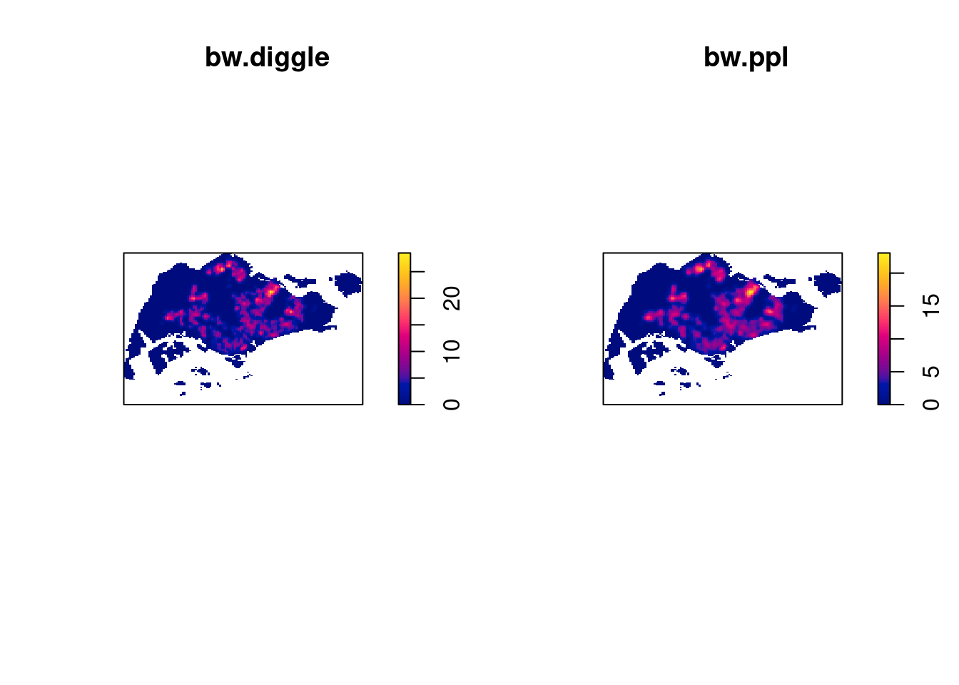
Working with different kernel methods
By default, the kernel method used in density.ppp() is gaussian. But there are three other options, namely: Epanechnikov, Quartic and Discs.
The code chunk below will be used to compute three more kernel density estimations by using these three kernel function.
These are interpolations to deal with areas that has less data.
If you use Gaussian, you sometimes get negative intensity values, so try to avoid it. Try quartic instead.
par(mfrow=c(2,2))
plot(density(childcareSG_ppp.km,
             sigma=bw.ppl,
             edge=TRUE,
             kernel="gaussian"),
     main="Gaussian")
plot(density(childcareSG_ppp.km,
             sigma=bw.ppl,
             edge=TRUE,
             kernel="epanechnikov"),
     main="Epanechnikov")
Warning in density.ppp(childcareSG_ppp.km, sigma = bw.ppl, edge = TRUE, :
Bandwidth selection will be based on Gaussian kernelplot(density(childcareSG_ppp.km,
sigma=bw.ppl,
edge=TRUE,
kernel="quartic"),
main="Quartic")Warning in density.ppp(childcareSG_ppp.km, sigma = bw.ppl, edge = TRUE, :
Bandwidth selection will be based on Gaussian kernelplot(density(childcareSG_ppp.km,
sigma=bw.ppl,
edge=TRUE,
kernel="disc"),
main="Disc")Warning in density.ppp(childcareSG_ppp.km, sigma = bw.ppl, edge = TRUE, :
Bandwidth selection will be based on Gaussian kernel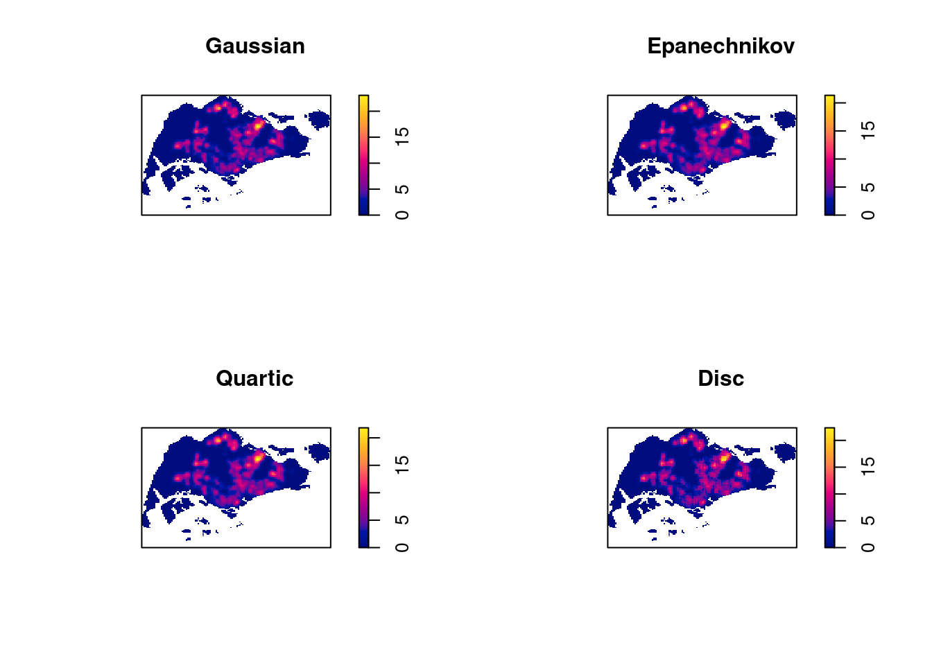
Manually setting the bandwidth
Since the unit of measurement has changed to kilometres, the sigma value used is 0.6 instead of 600 metres.
kde_childcareSG_600 <- density(childcareSG_ppp.km, sigma=0.6, edge=TRUE, kernel="gaussian")
plot(kde_childcareSG_600)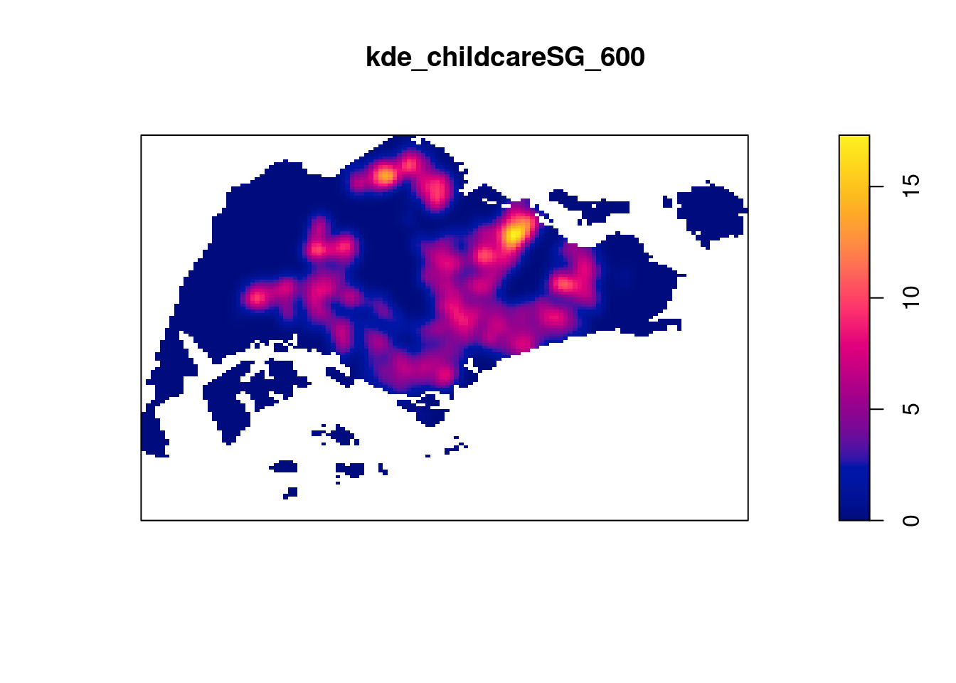
Why would you use fixed bandwidth?
This approach is appropriate in several situations, particularly when the underlying data is relatively uniform in its distribution (extremely unlikely unless the area of analysis is small) and when the focus is on identifying broad trends or when the study area does not exhibit significant variations in density.
How would you know if your data is highly skewed?
You can either visually inspect the plot, or use summary statistics.
quadrat.test(childcareSG_ppp)Warning: Some expected counts are small; chi^2 approximation may be inaccurate
    Chi-squared test of CSR using quadrat counts

data:  childcareSG_ppp
X2 = 676.18, df = 20, p-value < 2.2e-16
alternative hypothesis: two.sided

Quadrats: 21 tiles (irregular windows)
A significant result (low p-value) indicates that the points are not uniformly distributed and may be highly skewed, with clustering in certain areas.
Using adaptive bandwidth
kde_childcareSG_adaptive <- adaptive.density(childcareSG_ppp.km, method="kernel")
plot(kde_childcareSG_adaptive)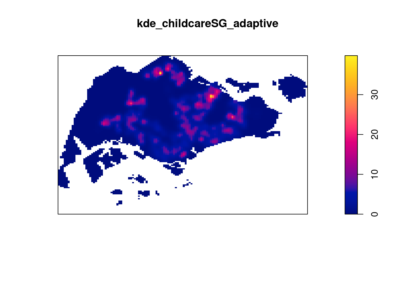
We can compare the fixed and adaptive kernel density estimation outputs by using the code chunk below.
Unlike fixed bandwidth, we adjust the area according to the density of points.
par(mfrow=c(1,2))
plot(kde_childcareSG.bw, main = "Fixed bandwidth")
plot(kde_childcareSG_adaptive, main = "Adaptive bandwidth")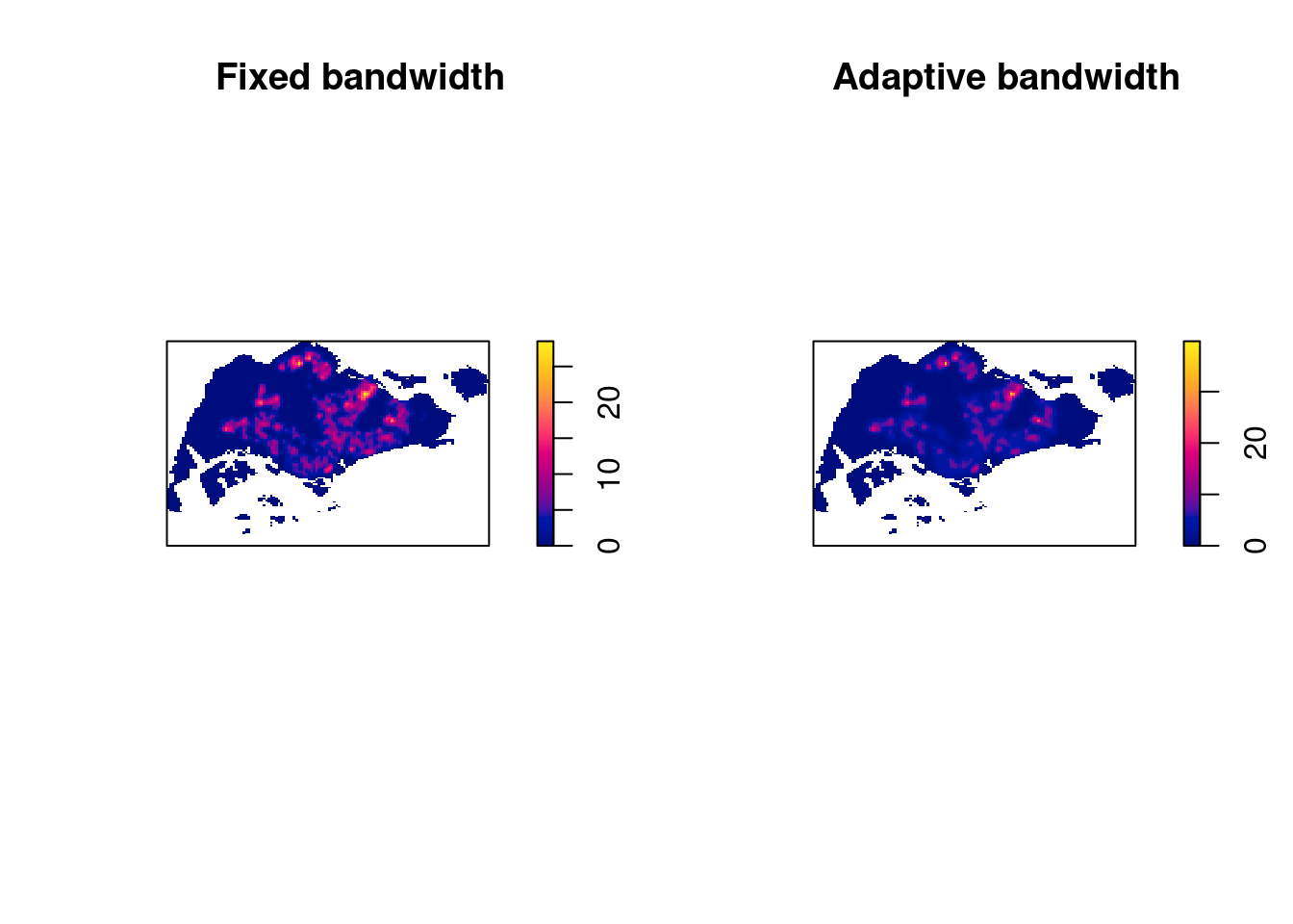
Converting KDE output into grid object
The result is the same, we just convert it so that it is suitable for mapping purposes.
gridded_kde_childcareSG_bw <- as(kde_childcareSG.bw, "SpatialGridDataFrame")
spplot(gridded_kde_childcareSG_bw)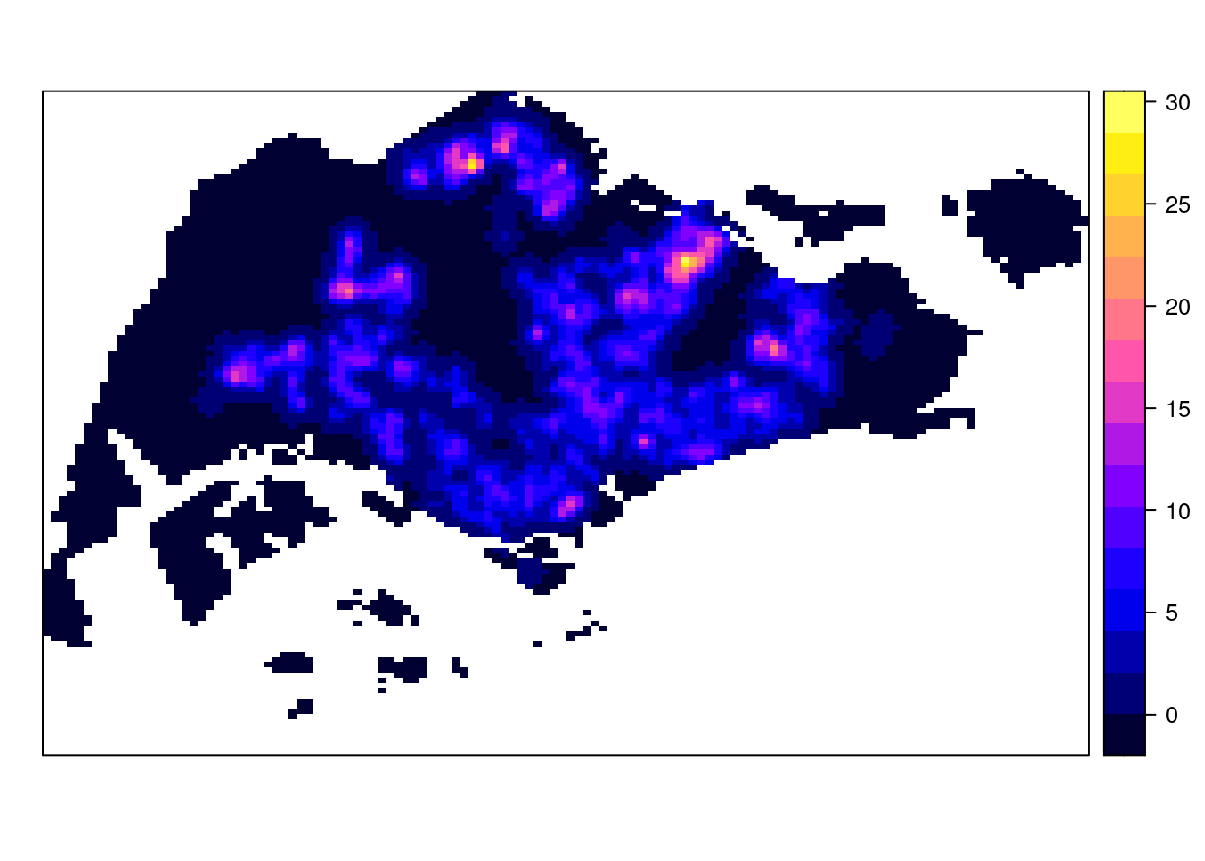
Next, we will convert the gridded kernel density objects into RasterLayer object by using raster() of raster package.
A raster is a type of data structure commonly used in Geographic Information Systems (GIS) to represent spatial data. It is a grid-based format that divides a geographic area into a matrix of cells or pixels, where each cell contains a value representing information such as elevation, temperature, land cover, or any other spatial attribute.
kde_childcareSG_bw_raster <- raster(kde_childcareSG.bw)Let us take a look at the properties of kde_childcareSG_bw_raster RasterLayer.
kde_childcareSG_bw_rasterclass : RasterLayer
dimensions : 128, 128, 16384 (nrow, ncol, ncell)
resolution : 0.4170614, 0.2647348 (x, y)
extent : 2.663926, 56.04779, 16.35798, 50.24403 (xmin, xmax, ymin, ymax)
crs : NA
source : memory
names : layer
values : -8.476185e-15, 28.51831 (min, max)Notice that the crs property is NA.
The code chunk below will be used to include the CRS information on kde_childcareSG_bw_raster RasterLayer.
projection(kde_childcareSG_bw_raster) <- CRS("+init=EPSG:3414")
kde_childcareSG_bw_raster
class : RasterLayer
dimensions : 128, 128, 16384 (nrow, ncol, ncell)
resolution : 0.4170614, 0.2647348 (x, y)
extent : 2.663926, 56.04779, 16.35798, 50.24403 (xmin, xmax, ymin, ymax)
crs : +proj=tmerc +lat_0=1.36666666666667 +lon_0=103.833333333333 +k=1 +x_0=28001.642 +y_0=38744.572 +ellps=WGS84 +units=m +no_defs
source : memory
names : layer
values : -8.476185e-15, 28.51831 (min, max)tm_shape(kde_childcareSG_bw_raster) +
tm_raster("layer", palette = "viridis") +
tm_layout(legend.position = c("right", "bottom"), frame = FALSE)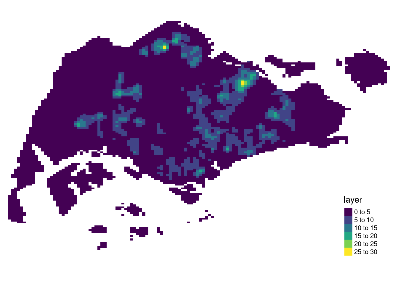
Notice that the raster values are encoded explicitly onto the raster pixel using the values in “v”” field.
Comparing Spatial Point Patterns using KDE
In this section, you will learn how to compare KDE of childcare at Ponggol, Tampines, Chua Chu Kang and Jurong West planning areas.
The code chunk below will be used to extract the target planning areas.
pg <- mpsz_sf %>%
  filter(PLN_AREA_N == "PUNGGOL")
tm <- mpsz_sf %>%
  filter(PLN_AREA_N == "TAMPINES")
ck <- mpsz_sf %>%
  filter(PLN_AREA_N == "CHOA CHU KANG")
jw <- mpsz_sf %>%
  filter(PLN_AREA_N == "JURONG WEST")
Plotting target planning areas:
par(mfrow=c(2,2))
plot(pg, main = "Ponggol")
Warning: plotting the first 9 out of 15 attributes; use max.plot = 15 to plot
all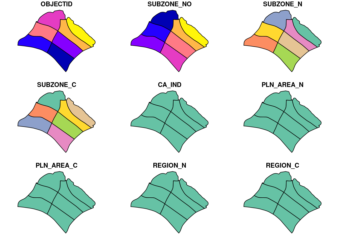
plot(tm, main = "Tampines")Warning: plotting the first 9 out of 15 attributes; use max.plot = 15 to plot
all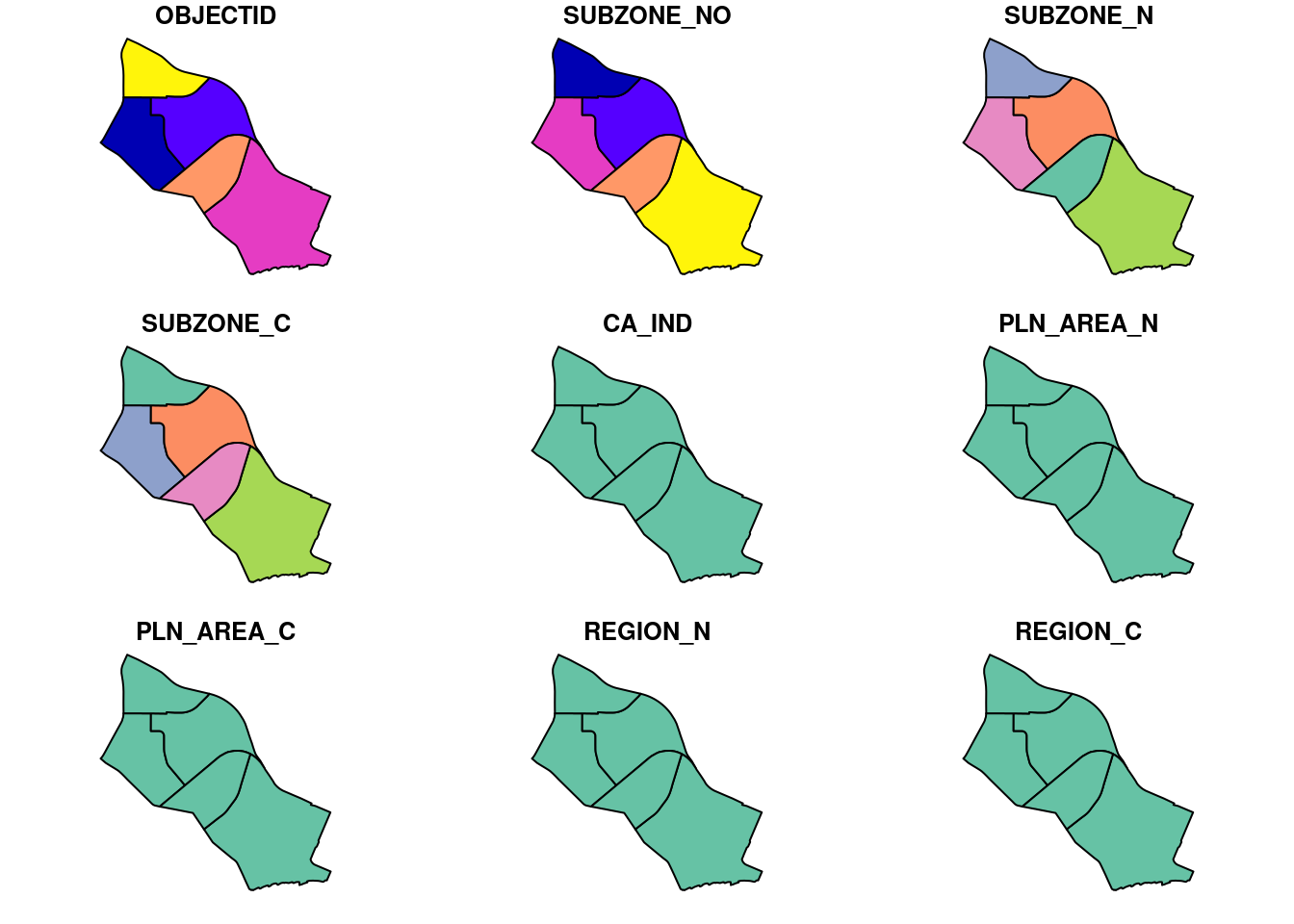
plot(ck, main = "Choa Chu Kang")Warning: plotting the first 10 out of 15 attributes; use max.plot = 15 to plot
all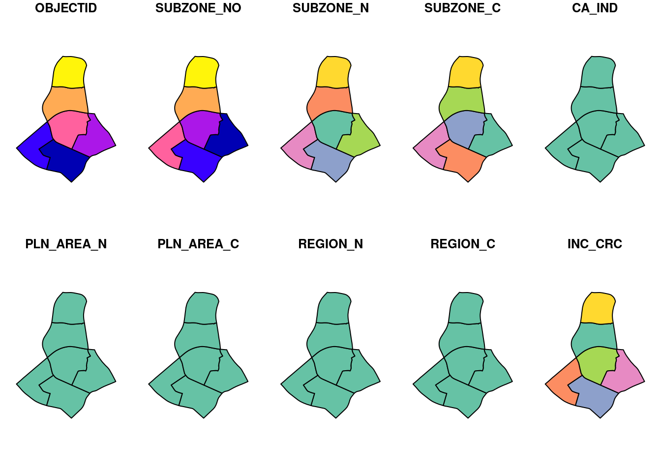
plot(jw, main = "Jurong West")Warning: plotting the first 9 out of 15 attributes; use max.plot = 15 to plot
all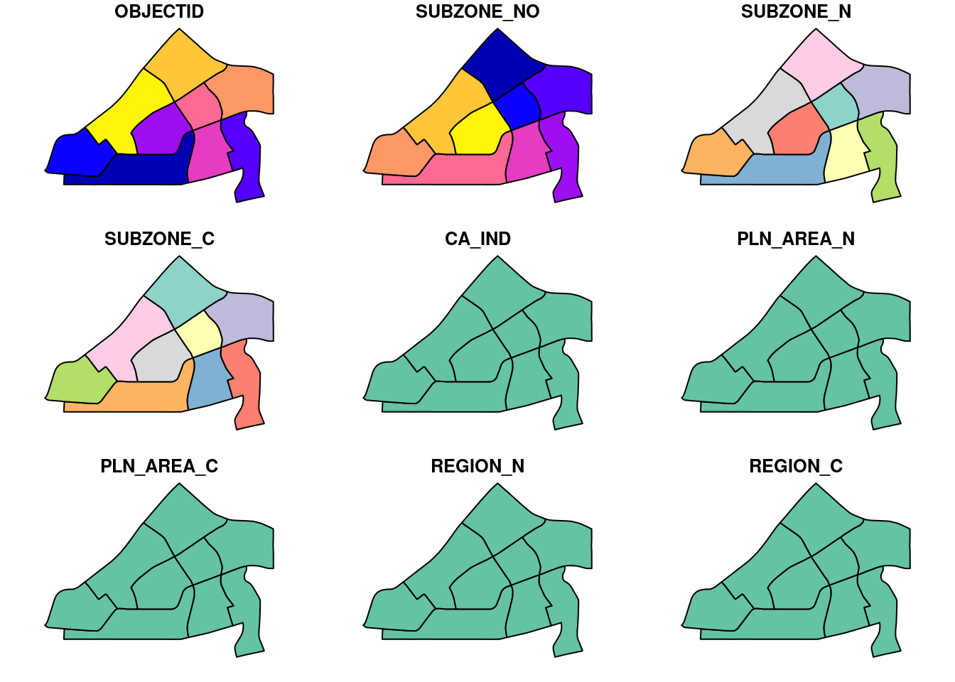
Now, we will convert these sf objects into owin objects that is required by spatstat.
pg_owin = as.owin(pg)
tm_owin = as.owin(tm)
ck_owin = as.owin(ck)
jw_owin = as.owin(jw)
By using the code chunk below, we are able to extract childcare that is within the specific region to do our analysis later on.
Now why would you bother to split them up? To analyse spatial randomness it is essential to exclude regions like the airport where there are no childcare centres.
childcare_pg_ppp = childcare_ppp_jit[pg_owin]
childcare_tm_ppp = childcare_ppp_jit[tm_owin]
childcare_ck_ppp = childcare_ppp_jit[ck_owin]
childcare_jw_ppp = childcare_ppp_jit[jw_owin]
Next, rescale.ppp() function is used to trasnform the unit of measurement from metre to kilometre.
childcare_pg_ppp.km = rescale.ppp(childcare_pg_ppp, 1000, "km")
childcare_tm_ppp.km = rescale.ppp(childcare_tm_ppp, 1000, "km")
childcare_ck_ppp.km = rescale.ppp(childcare_ck_ppp, 1000, "km")
childcare_jw_ppp.km = rescale.ppp(childcare_jw_ppp, 1000, "km")
The code chunk below is used to plot these four study areas and the locations of the childcare centres.
par(mfrow=c(2,2))
plot(childcare_pg_ppp.km, main="Punggol")
Warning in default.charmap(ntypes, chars): Too many types to display every type
as a different characterWarning: Only 10 out of 61 symbols are shown in the symbol mapplot(childcare_tm_ppp.km, main="Tampines")Warning in default.charmap(ntypes, chars): Too many types to display every type
as a different characterWarning: Only 10 out of 89 symbols are shown in the symbol mapplot(childcare_ck_ppp.km, main="Choa Chu Kang")Warning in default.charmap(ntypes, chars): Too many types to display every type
as a different characterWarning: Only 10 out of 61 symbols are shown in the symbol mapplot(childcare_jw_ppp.km, main="Jurong West")Warning in default.charmap(ntypes, chars): Too many types to display every type
as a different characterWarning: Only 10 out of 88 symbols are shown in the symbol map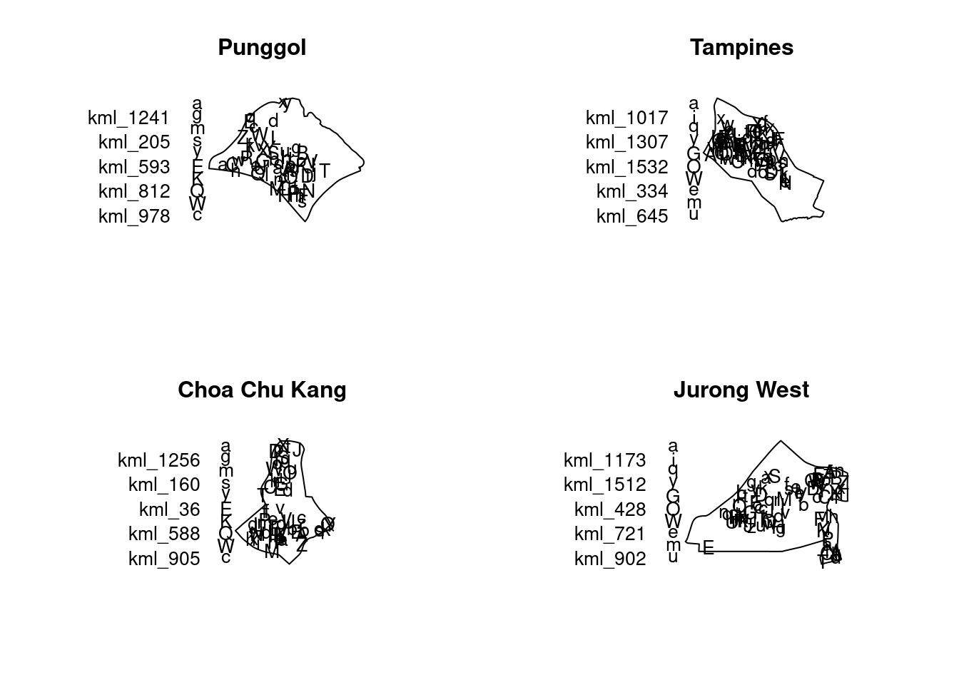
The code chunk below will be used to compute the KDE of these four planning area. bw.diggle method is used to derive the bandwidth of each
par(mfrow=c(2,2))
plot(density(childcare_pg_ppp.km,
             sigma=bw.diggle,
             edge=TRUE,
             kernel="gaussian"),
     main="Punggol")
plot(density(childcare_tm_ppp.km,
             sigma=bw.diggle,
             edge=TRUE,
             kernel="gaussian"),
     main="Tempines")
plot(density(childcare_ck_ppp.km,
             sigma=bw.diggle,
             edge=TRUE,
             kernel="gaussian"),
     main="Choa Chu Kang")
plot(density(childcare_jw_ppp.km,
             sigma=bw.diggle,
             edge=TRUE,
             kernel="gaussian"),
     main="JUrong West")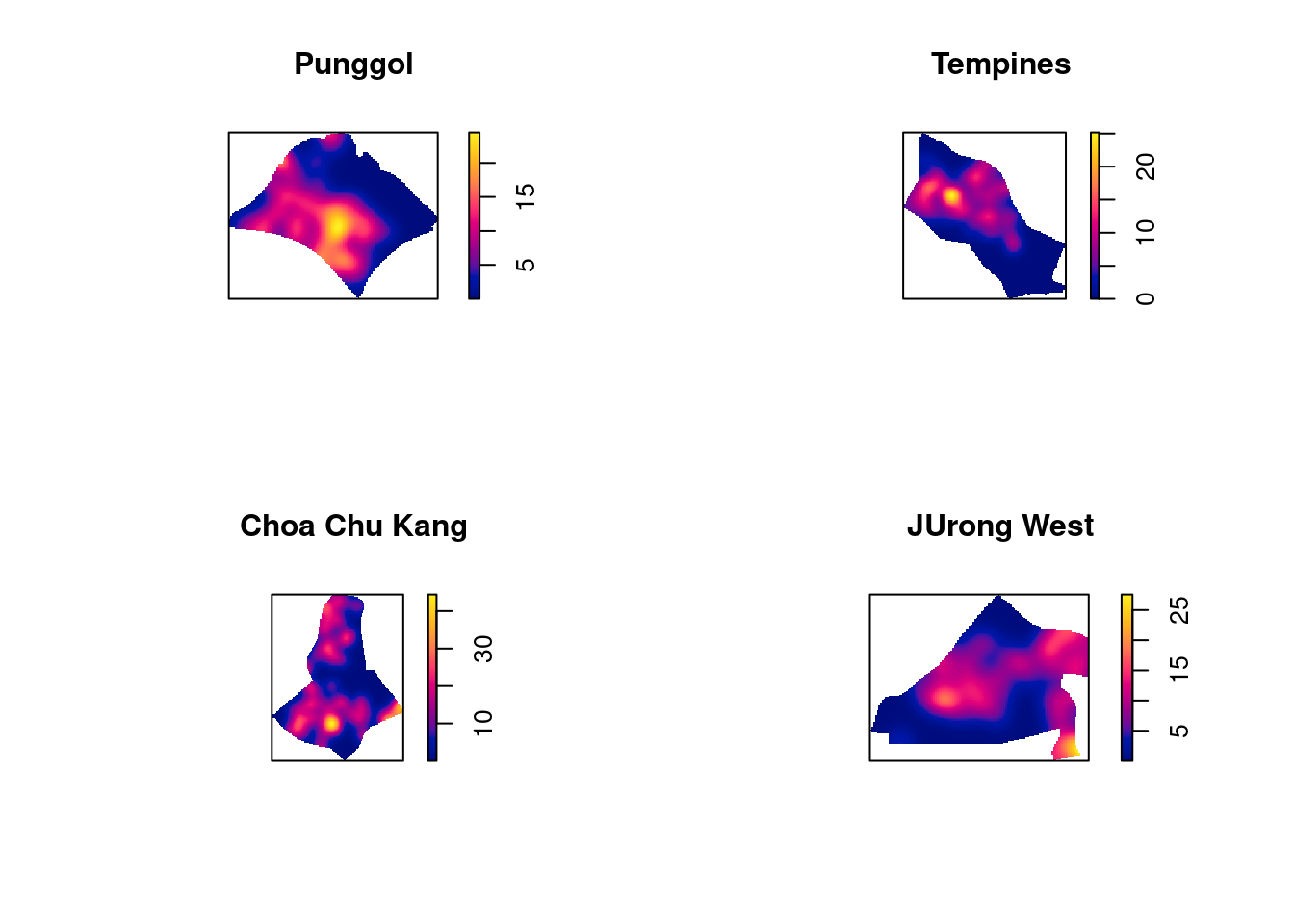
For comparison purposes, we will use 250m as the bandwidth.
par(mfrow=c(2,2))
plot(density(childcare_ck_ppp.km,
             sigma=0.25,
             edge=TRUE,
             kernel="gaussian"),
     main="Choa Chu Kang")
plot(density(childcare_jw_ppp.km,
             sigma=0.25,
             edge=TRUE,
             kernel="gaussian"),
     main="Jurong West")
plot(density(childcare_pg_ppp.km,
             sigma=0.25,
             edge=TRUE,
             kernel="gaussian"),
     main="Punggol")
plot(density(childcare_tm_ppp.km,
             sigma=0.25,
             edge=TRUE,
             kernel="gaussian"),
     main="Tampines")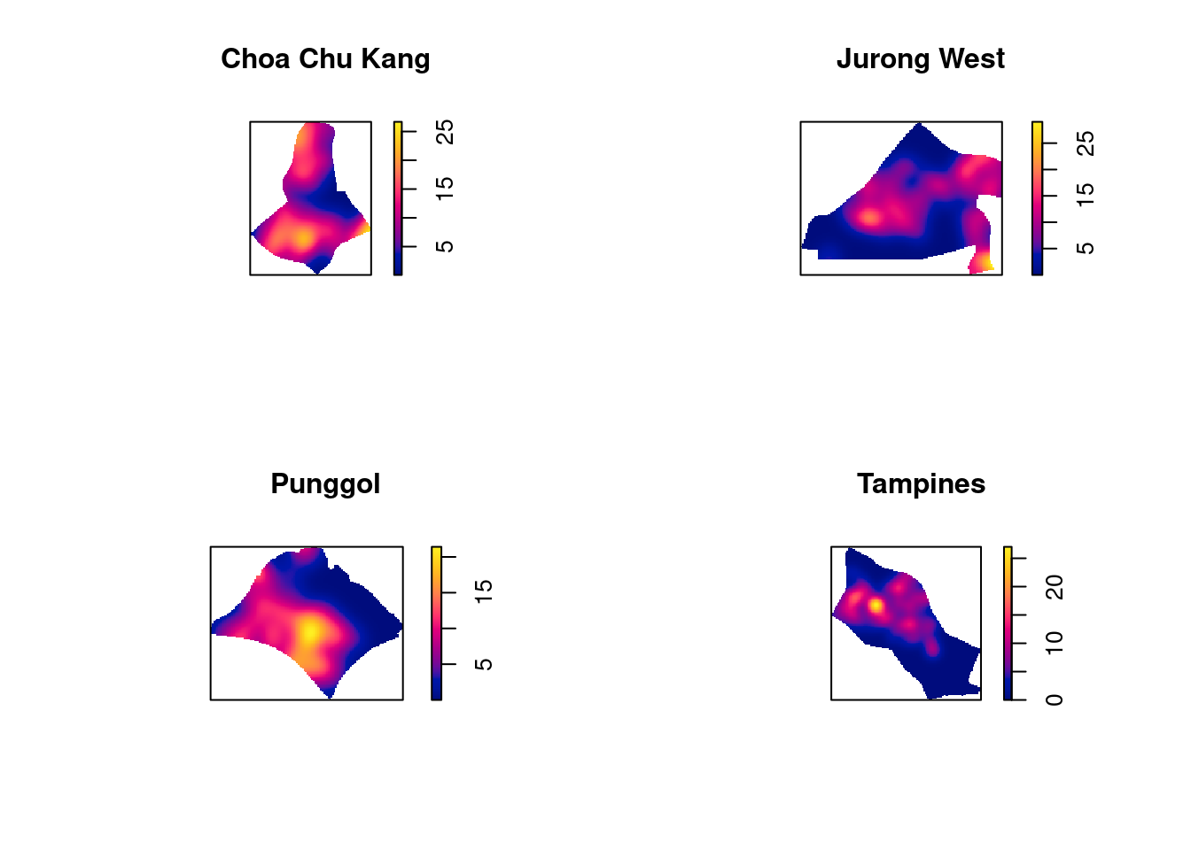
Nearest neighbour analysis
In this section, we will perform the Clark-Evans test of aggregation for a spatial point pattern by using clarkevans.test() of statspat.
The test hypotheses are:
Ho = The distribution of childcare services are randomly distributed.
H1= The distribution of childcare services are not randomly distributed.
The 95% confident interval will be used.
clarkevans.test(childcareSG_ppp,
                correction="none",
                clipregion="sg_owin",
                alternative=c("clustered"),
                nsim=99)
    Clark-Evans test
    No edge correction
    Z-test

data:  childcareSG_ppp
R = 0.55631, p-value < 2.2e-16
alternative hypothesis: clustered (R < 1)
R = 0.55631:
The R value is the Clark-Evans ratio, which compares the observed average nearest neighbor distance to the expected nearest neighbor distance for a random distribution.
R = 1 indicates a random distribution.
R < 1 indicates clustering (i.e., the points are closer to each other than expected under randomness).
R > 1 indicates dispersion (i.e., the points are more evenly spread out than expected under randomness).
In this case, R = 0.55631, which is significantly less than 1, indicating that the childcare services are clustered.
p-value < 2.2e-16:
The p-value represents the probability of observing such a clustered pattern under the null hypothesis of randomness.
A p-value less than the significance level (α = 0.05) allows us to reject the null hypothesis. In this case, the p-value is extremely small (essentially zero), far below the 0.05 threshold.
Conclusion:
Since R < 1 and the p-value is extremely small, we reject the null hypothesis.
This means we have strong evidence to conclude that the distribution of childcare services in Singapore is not randomly distributed. Instead, the distribution is clustered—that is, the childcare services tend to be closer together than what would be expected under a random spatial distribution.
In the code chunk below, clarkevans.test() of spatstat is used to performs Clark-Evans test of aggregation for childcare centre in Choa Chu Kang planning area.
Null Hypothesis (Ho): The distribution of childcare services is randomly distributed (CSR, Complete Spatial Randomness).
Alternative Hypothesis (H1): The distribution of childcare services is not randomly distributed. This includes both possibilities: the points may be either clustered (R < 1) or regularly spaced (R > 1). If the index is close or equal to 1, the patterns exhibit randomness.
Regularity (also known as dispersion) in the context of spatial point patterns refers to a distribution where points are more evenly spaced than would be expected under complete spatial randomness (CSR). Essentially, regularity or dispersion implies that points are systematically spread out, avoiding clustering, and often maintaining a more uniform distance from each other.
clarkevans.test(childcare_ck_ppp,
                correction="none",
                clipregion=NULL,
                alternative=c("two.sided"),
                nsim=999)
    Clark-Evans test
    No edge correction
    Z-test

data:  childcare_ck_ppp
R = 0.91837, p-value = 0.2226
alternative hypothesis: two-sided
Since the p-value is large (0.4801), you fail to reject the null hypothesis (Ho). This means that the observed pattern of childcare services in
childcare_ck_pppis not significantly different from random.Conclusion: The distribution of childcare services is consistent with complete spatial randomness (CSR). There is no statistically significant evidence to suggest that the points are either clustered or regularly spaced.
Note: Since you are using more simulation iterations, the time taken to run the tests will be longer. Since this is essentially Monte Carlo simulation, to satisfy a 95% confidence interval, we need a minimum of 39 for convergence. 99, 199, 999 are common values. We need a greater amount to achieve a more stable result. Note that 99 means that you are running it 100 times.
Note that it is typical for randomness to occur when the area of analysis is high. It is important to figure out that at what distance does clustering occur and at what distance randomness starts to appear again. This can be done using the L function. We can further modify the L function to make it from a diagonal to a straight line. We have lots of different functions, like G function (zonal - within a ring buffer, how many points are there, and slowly draw more and more bigger rings, so unlike K function it is not cumulative, there is no straight version of it) or K function (the L function is the same as the K function except a transformation is applied to the result to make the graph straight, making it easier to interpret). Each employ a different shape but they are all distance based. Some analyse distances zone by zone while some are cumulative.
Also, if you need a constant result, you have to set the seed. You only have to set the seed once at the top of the document for maximum reproducibility.
1. One-Sided Test (Clustered or Dispersed):
a. Testing for Clustering:
When to Use:
Use the one-sided test with the
alternative = "clustered"option when you have a prior expectation or hypothesis that the points are more likely to be clustered rather than dispersed.Example: If you are studying the distribution of businesses that tend to cluster in urban centers, you might hypothesize that these businesses are more likely to be clustered due to factors like proximity to customers or each other.
Interpretation:
R < 1: Supports the hypothesis that the points are clustered.
R > 1: Would indicate regular spacing, but this result would be unexpected and not directly tested in this scenario.
b. Testing for Regular Spacing (Dispersion):
When to Use:
Use the one-sided test with
alternative = "regular"(or sometimesalternative = "dispersed") when you suspect that points are more regularly spaced, perhaps due to competition, territoriality, or other factors that push points apart.Example: In ecology, if you are studying tree locations in a forest where trees are expected to be evenly spaced due to competition for resources, you might test for regular spacing.
Interpretation:
R > 1: Supports the hypothesis that the points are regularly spaced.
R < 1: Would indicate clustering, but this result would be unexpected and not directly tested in this scenario.
2. Two-Sided Test:
When to Use:
Use the two-sided test with
alternative = "two.sided"when you do not have a specific expectation about whether the points are clustered or dispersed, and you want to test for any significant deviation from complete spatial randomness (CSR).This is appropriate when you are exploring the data without a strong prior hypothesis about the nature of the spatial distribution.
Example: If you are conducting an exploratory analysis of a new dataset and are unsure whether the points might be clustered or dispersed, the two-sided test is appropriate.
Interpretation:
R < 1 with a significant p-value: Indicates clustering.
R > 1 with a significant p-value: Indicates regular spacing.
R ≈ 1 with a non-significant p-value: Indicates a random distribution.
3. Choosing Edge Correction:
Edge Correction (
correctionparameter):Use edge correction if your study area is bounded (e.g., a city boundary, nature reserve) and the points near the boundary might have fewer neighbors simply due to being near the edge. This correction helps adjust for this bias.
If your study area is very large or if edge effects are not a concern, you might choose
correction = "none", as in your examples.
clarkevans.test(childcare_tm_ppp,
                correction="none",
                clipregion=NULL,
                alternative=c("two.sided"),
                nsim=999)
    Clark-Evans test
    No edge correction
    Z-test

data:  childcare_tm_ppp
R = 0.77178, p-value = 3.806e-05
alternative hypothesis: two-sided
Since the p-value is small (0.0004794), you reject the null hypothesis (Ho). This means that the observed pattern of childcare services in
childcare_tm_pppis significantly different from random.Conclusion: The distribution of childcare services is consistent with complete spatial randomness (CSR). There is statistically significant evidence to suggest that the points are either clustered or regularly spaced.