pacman::p_load(olsrr, corrplot, ggpubr, sf, spdep, GWmodel, tmap, tidyverse, gtsummary)Hands-on Exercise 9
Calibrating Hedonic Pricing Model for Private High-Rise Property with GWR Method
GWR is a method that helps us understand how different factors (like weather, population, or physical surroundings) affect something we’re interested in (like the price of a condo). In this exercise, we’ll use GWR to create a hedonic pricing model for Singapore condos in 2015. This model will predict condo prices based on things like the building’s size, location, and other features.
Importing packages
GWModel
GWmodel is a tool that helps us analyze data based on location. It uses different statistical methods to understand patterns and relationships in data. For example, it can help us find areas with similar characteristics or predict values based on location. These results can be visualized on a map to help us see trends and make better decisions.
Importing data
mpsz = st_read(dsn = "data/geospatial", layer = "MP14_SUBZONE_WEB_PL")Reading layer `MP14_SUBZONE_WEB_PL' from data source
`/home/tropicbliss/GitHub/quarto-project/Hands-on_Ex/Hands-on_Ex09/data/geospatial'
using driver `ESRI Shapefile'
Simple feature collection with 323 features and 15 fields
Geometry type: MULTIPOLYGON
Dimension: XY
Bounding box: xmin: 2667.538 ymin: 15748.72 xmax: 56396.44 ymax: 50256.33
Projected CRS: SVY21condo_resale = read_csv("data/aspatial/Condo_resale_2015.csv")Rows: 1436 Columns: 23
── Column specification ────────────────────────────────────────────────────────
Delimiter: ","
dbl (23): LATITUDE, LONGITUDE, POSTCODE, SELLING_PRICE, AREA_SQM, AGE, PROX_...
ℹ Use `spec()` to retrieve the full column specification for this data.
ℹ Specify the column types or set `show_col_types = FALSE` to quiet this message.Data wrangling
Spatial data
Now, we need to change the projection.
mpsz_svy21 <- st_transform(mpsz, 3414)
st_crs(mpsz_svy21)Coordinate Reference System:
User input: EPSG:3414
wkt:
PROJCRS["SVY21 / Singapore TM",
BASEGEOGCRS["SVY21",
DATUM["SVY21",
ELLIPSOID["WGS 84",6378137,298.257223563,
LENGTHUNIT["metre",1]]],
PRIMEM["Greenwich",0,
ANGLEUNIT["degree",0.0174532925199433]],
ID["EPSG",4757]],
CONVERSION["Singapore Transverse Mercator",
METHOD["Transverse Mercator",
ID["EPSG",9807]],
PARAMETER["Latitude of natural origin",1.36666666666667,
ANGLEUNIT["degree",0.0174532925199433],
ID["EPSG",8801]],
PARAMETER["Longitude of natural origin",103.833333333333,
ANGLEUNIT["degree",0.0174532925199433],
ID["EPSG",8802]],
PARAMETER["Scale factor at natural origin",1,
SCALEUNIT["unity",1],
ID["EPSG",8805]],
PARAMETER["False easting",28001.642,
LENGTHUNIT["metre",1],
ID["EPSG",8806]],
PARAMETER["False northing",38744.572,
LENGTHUNIT["metre",1],
ID["EPSG",8807]]],
CS[Cartesian,2],
AXIS["northing (N)",north,
ORDER[1],
LENGTHUNIT["metre",1]],
AXIS["easting (E)",east,
ORDER[2],
LENGTHUNIT["metre",1]],
USAGE[
SCOPE["Cadastre, engineering survey, topographic mapping."],
AREA["Singapore - onshore and offshore."],
BBOX[1.13,103.59,1.47,104.07]],
ID["EPSG",3414]]Now, we will check the extent (spatial boundaries or area covered by a particular feature) by using st_bbox.
st_bbox(mpsz_svy21) xmin ymin xmax ymax
2667.538 15748.721 56396.440 50256.334 Aspatial data
Let’s take a look at all the available columns of the condo data.
glimpse(condo_resale)Rows: 1,436
Columns: 23
$ LATITUDE <dbl> 1.287145, 1.328698, 1.313727, 1.308563, 1.321437,…
$ LONGITUDE <dbl> 103.7802, 103.8123, 103.7971, 103.8247, 103.9505,…
$ POSTCODE <dbl> 118635, 288420, 267833, 258380, 467169, 466472, 3…
$ SELLING_PRICE <dbl> 3000000, 3880000, 3325000, 4250000, 1400000, 1320…
$ AREA_SQM <dbl> 309, 290, 248, 127, 145, 139, 218, 141, 165, 168,…
$ AGE <dbl> 30, 32, 33, 7, 28, 22, 24, 24, 27, 31, 17, 22, 6,…
$ PROX_CBD <dbl> 7.941259, 6.609797, 6.898000, 4.038861, 11.783402…
$ PROX_CHILDCARE <dbl> 0.16597932, 0.28027246, 0.42922669, 0.39473543, 0…
$ PROX_ELDERLYCARE <dbl> 2.5198118, 1.9333338, 0.5021395, 1.9910316, 1.121…
$ PROX_URA_GROWTH_AREA <dbl> 6.618741, 7.505109, 6.463887, 4.906512, 6.410632,…
$ PROX_HAWKER_MARKET <dbl> 1.76542207, 0.54507614, 0.37789301, 1.68259969, 0…
$ PROX_KINDERGARTEN <dbl> 0.05835552, 0.61592412, 0.14120309, 0.38200076, 0…
$ PROX_MRT <dbl> 0.5607188, 0.6584461, 0.3053433, 0.6910183, 0.528…
$ PROX_PARK <dbl> 1.1710446, 0.1992269, 0.2779886, 0.9832843, 0.116…
$ PROX_PRIMARY_SCH <dbl> 1.6340256, 0.9747834, 1.4715016, 1.4546324, 0.709…
$ PROX_TOP_PRIMARY_SCH <dbl> 3.3273195, 0.9747834, 1.4715016, 2.3006394, 0.709…
$ PROX_SHOPPING_MALL <dbl> 2.2102717, 2.9374279, 1.2256850, 0.3525671, 1.307…
$ PROX_SUPERMARKET <dbl> 0.9103958, 0.5900617, 0.4135583, 0.4162219, 0.581…
$ PROX_BUS_STOP <dbl> 0.10336166, 0.28673408, 0.28504777, 0.29872340, 0…
$ NO_Of_UNITS <dbl> 18, 20, 27, 30, 30, 31, 32, 32, 32, 32, 34, 34, 3…
$ FAMILY_FRIENDLY <dbl> 0, 0, 0, 0, 0, 1, 1, 0, 1, 1, 0, 0, 0, 0, 0, 0, 0…
$ FREEHOLD <dbl> 1, 1, 1, 1, 1, 1, 1, 1, 1, 0, 1, 1, 1, 1, 1, 1, 1…
$ LEASEHOLD_99YR <dbl> 0, 0, 0, 0, 0, 0, 0, 0, 0, 0, 0, 0, 0, 0, 0, 0, 0…head(condo_resale$LONGITUDE) # see the data in XCOORD column[1] 103.7802 103.8123 103.7971 103.8247 103.9505 103.9386head(condo_resale$LATITUDE) # see the data in YCOORD column[1] 1.287145 1.328698 1.313727 1.308563 1.321437 1.314198summary(condo_resale) LATITUDE LONGITUDE POSTCODE SELLING_PRICE
Min. :1.240 Min. :103.7 Min. : 18965 Min. : 540000
1st Qu.:1.309 1st Qu.:103.8 1st Qu.:259849 1st Qu.: 1100000
Median :1.328 Median :103.8 Median :469298 Median : 1383222
Mean :1.334 Mean :103.8 Mean :440439 Mean : 1751211
3rd Qu.:1.357 3rd Qu.:103.9 3rd Qu.:589486 3rd Qu.: 1950000
Max. :1.454 Max. :104.0 Max. :828833 Max. :18000000
AREA_SQM AGE PROX_CBD PROX_CHILDCARE
Min. : 34.0 Min. : 0.00 Min. : 0.3869 Min. :0.004927
1st Qu.:103.0 1st Qu.: 5.00 1st Qu.: 5.5574 1st Qu.:0.174481
Median :121.0 Median :11.00 Median : 9.3567 Median :0.258135
Mean :136.5 Mean :12.14 Mean : 9.3254 Mean :0.326313
3rd Qu.:156.0 3rd Qu.:18.00 3rd Qu.:12.6661 3rd Qu.:0.368293
Max. :619.0 Max. :37.00 Max. :19.1804 Max. :3.465726
PROX_ELDERLYCARE PROX_URA_GROWTH_AREA PROX_HAWKER_MARKET PROX_KINDERGARTEN
Min. :0.05451 Min. :0.2145 Min. :0.05182 Min. :0.004927
1st Qu.:0.61254 1st Qu.:3.1643 1st Qu.:0.55245 1st Qu.:0.276345
Median :0.94179 Median :4.6186 Median :0.90842 Median :0.413385
Mean :1.05351 Mean :4.5981 Mean :1.27987 Mean :0.458903
3rd Qu.:1.35122 3rd Qu.:5.7550 3rd Qu.:1.68578 3rd Qu.:0.578474
Max. :3.94916 Max. :9.1554 Max. :5.37435 Max. :2.229045
PROX_MRT PROX_PARK PROX_PRIMARY_SCH PROX_TOP_PRIMARY_SCH
Min. :0.05278 Min. :0.02906 Min. :0.07711 Min. :0.07711
1st Qu.:0.34646 1st Qu.:0.26211 1st Qu.:0.44024 1st Qu.:1.34451
Median :0.57430 Median :0.39926 Median :0.63505 Median :1.88213
Mean :0.67316 Mean :0.49802 Mean :0.75471 Mean :2.27347
3rd Qu.:0.84844 3rd Qu.:0.65592 3rd Qu.:0.95104 3rd Qu.:2.90954
Max. :3.48037 Max. :2.16105 Max. :3.92899 Max. :6.74819
PROX_SHOPPING_MALL PROX_SUPERMARKET PROX_BUS_STOP NO_Of_UNITS
Min. :0.0000 Min. :0.0000 Min. :0.001595 Min. : 18.0
1st Qu.:0.5258 1st Qu.:0.3695 1st Qu.:0.098356 1st Qu.: 188.8
Median :0.9357 Median :0.5687 Median :0.151710 Median : 360.0
Mean :1.0455 Mean :0.6141 Mean :0.193974 Mean : 409.2
3rd Qu.:1.3994 3rd Qu.:0.7862 3rd Qu.:0.220466 3rd Qu.: 590.0
Max. :3.4774 Max. :2.2441 Max. :2.476639 Max. :1703.0
FAMILY_FRIENDLY FREEHOLD LEASEHOLD_99YR
Min. :0.0000 Min. :0.0000 Min. :0.0000
1st Qu.:0.0000 1st Qu.:0.0000 1st Qu.:0.0000
Median :0.0000 Median :0.0000 Median :0.0000
Mean :0.4868 Mean :0.4227 Mean :0.4882
3rd Qu.:1.0000 3rd Qu.:1.0000 3rd Qu.:1.0000
Max. :1.0000 Max. :1.0000 Max. :1.0000 Next, we will convert the CSV into an SFO, while projecting into SVY21.
condo_resale.sf <- st_as_sf(condo_resale,
coords = c("LONGITUDE", "LATITUDE"),
crs=4326) %>%
st_transform(crs=3414)head(condo_resale.sf)Simple feature collection with 6 features and 21 fields
Geometry type: POINT
Dimension: XY
Bounding box: xmin: 22085.12 ymin: 29951.54 xmax: 41042.56 ymax: 34546.2
Projected CRS: SVY21 / Singapore TM
# A tibble: 6 × 22
POSTCODE SELLING_PRICE AREA_SQM AGE PROX_CBD PROX_CHILDCARE PROX_ELDERLYCARE
<dbl> <dbl> <dbl> <dbl> <dbl> <dbl> <dbl>
1 118635 3000000 309 30 7.94 0.166 2.52
2 288420 3880000 290 32 6.61 0.280 1.93
3 267833 3325000 248 33 6.90 0.429 0.502
4 258380 4250000 127 7 4.04 0.395 1.99
5 467169 1400000 145 28 11.8 0.119 1.12
6 466472 1320000 139 22 10.3 0.125 0.789
# ℹ 15 more variables: PROX_URA_GROWTH_AREA <dbl>, PROX_HAWKER_MARKET <dbl>,
# PROX_KINDERGARTEN <dbl>, PROX_MRT <dbl>, PROX_PARK <dbl>,
# PROX_PRIMARY_SCH <dbl>, PROX_TOP_PRIMARY_SCH <dbl>,
# PROX_SHOPPING_MALL <dbl>, PROX_SUPERMARKET <dbl>, PROX_BUS_STOP <dbl>,
# NO_Of_UNITS <dbl>, FAMILY_FRIENDLY <dbl>, FREEHOLD <dbl>,
# LEASEHOLD_99YR <dbl>, geometry <POINT [m]>Exploratory Data Analysis
Plotting the distribution of selling price
ggplot(data=condo_resale.sf, aes(x=`SELLING_PRICE`)) +
geom_histogram(bins=20, color="black", fill="light blue")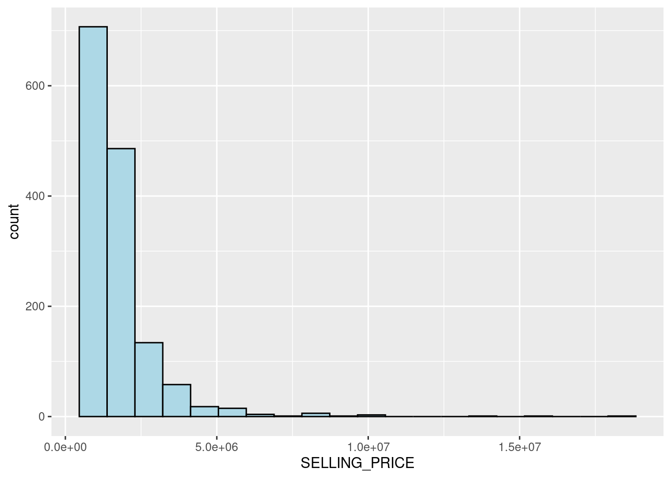
Since the figure shows a right-skewed distribution, this means that more condominium units were transacted at relatively low prices.
We can try to normalise the skewed distribution using log transformation since we assume that the data follows a normal distribution.
condo_resale.sf <- condo_resale.sf %>%
mutate(`LOG_SELLING_PRICE` = log(SELLING_PRICE))ggplot(data=condo_resale.sf, aes(x=`LOG_SELLING_PRICE`)) +
geom_histogram(bins=20, color="black", fill="light blue")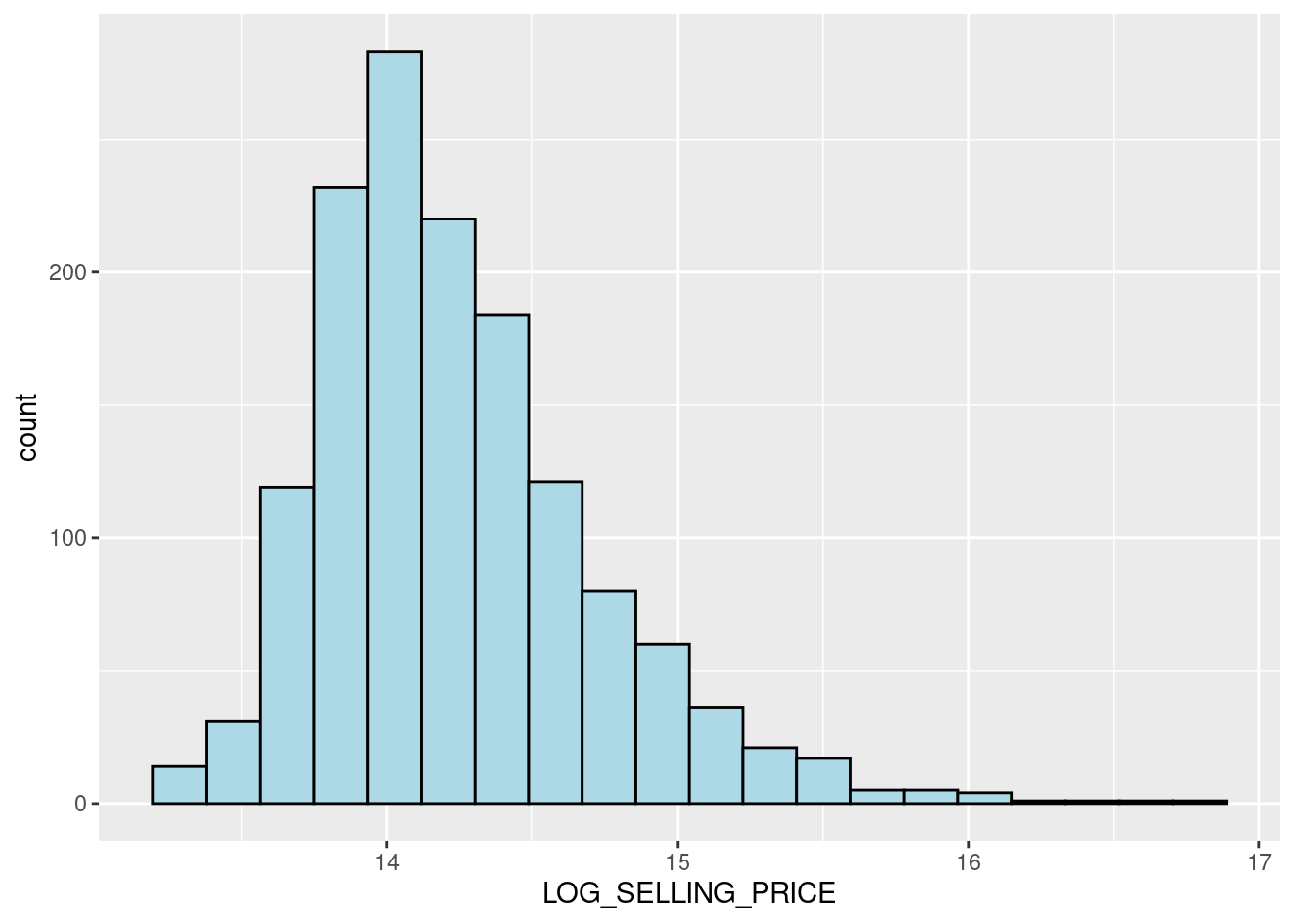
Notice that the distribution is relatively less skewed after the transformation.
Plotting multiple histograms (trellis plot) for each variable
AREA_SQM <- ggplot(data=condo_resale.sf, aes(x= `AREA_SQM`)) +
geom_histogram(bins=20, color="black", fill="light blue")
AGE <- ggplot(data=condo_resale.sf, aes(x= `AGE`)) +
geom_histogram(bins=20, color="black", fill="light blue")
PROX_CBD <- ggplot(data=condo_resale.sf, aes(x= `PROX_CBD`)) +
geom_histogram(bins=20, color="black", fill="light blue")
PROX_CHILDCARE <- ggplot(data=condo_resale.sf, aes(x= `PROX_CHILDCARE`)) +
geom_histogram(bins=20, color="black", fill="light blue")
PROX_ELDERLYCARE <- ggplot(data=condo_resale.sf, aes(x= `PROX_ELDERLYCARE`)) +
geom_histogram(bins=20, color="black", fill="light blue")
PROX_URA_GROWTH_AREA <- ggplot(data=condo_resale.sf,
aes(x= `PROX_URA_GROWTH_AREA`)) +
geom_histogram(bins=20, color="black", fill="light blue")
PROX_HAWKER_MARKET <- ggplot(data=condo_resale.sf, aes(x= `PROX_HAWKER_MARKET`)) +
geom_histogram(bins=20, color="black", fill="light blue")
PROX_KINDERGARTEN <- ggplot(data=condo_resale.sf, aes(x= `PROX_KINDERGARTEN`)) +
geom_histogram(bins=20, color="black", fill="light blue")
PROX_MRT <- ggplot(data=condo_resale.sf, aes(x= `PROX_MRT`)) +
geom_histogram(bins=20, color="black", fill="light blue")
PROX_PARK <- ggplot(data=condo_resale.sf, aes(x= `PROX_PARK`)) +
geom_histogram(bins=20, color="black", fill="light blue")
PROX_PRIMARY_SCH <- ggplot(data=condo_resale.sf, aes(x= `PROX_PRIMARY_SCH`)) +
geom_histogram(bins=20, color="black", fill="light blue")
PROX_TOP_PRIMARY_SCH <- ggplot(data=condo_resale.sf,
aes(x= `PROX_TOP_PRIMARY_SCH`)) +
geom_histogram(bins=20, color="black", fill="light blue")
ggarrange(AREA_SQM, AGE, PROX_CBD, PROX_CHILDCARE, PROX_ELDERLYCARE,
PROX_URA_GROWTH_AREA, PROX_HAWKER_MARKET, PROX_KINDERGARTEN, PROX_MRT,
PROX_PARK, PROX_PRIMARY_SCH, PROX_TOP_PRIMARY_SCH,
ncol = 3, nrow = 4)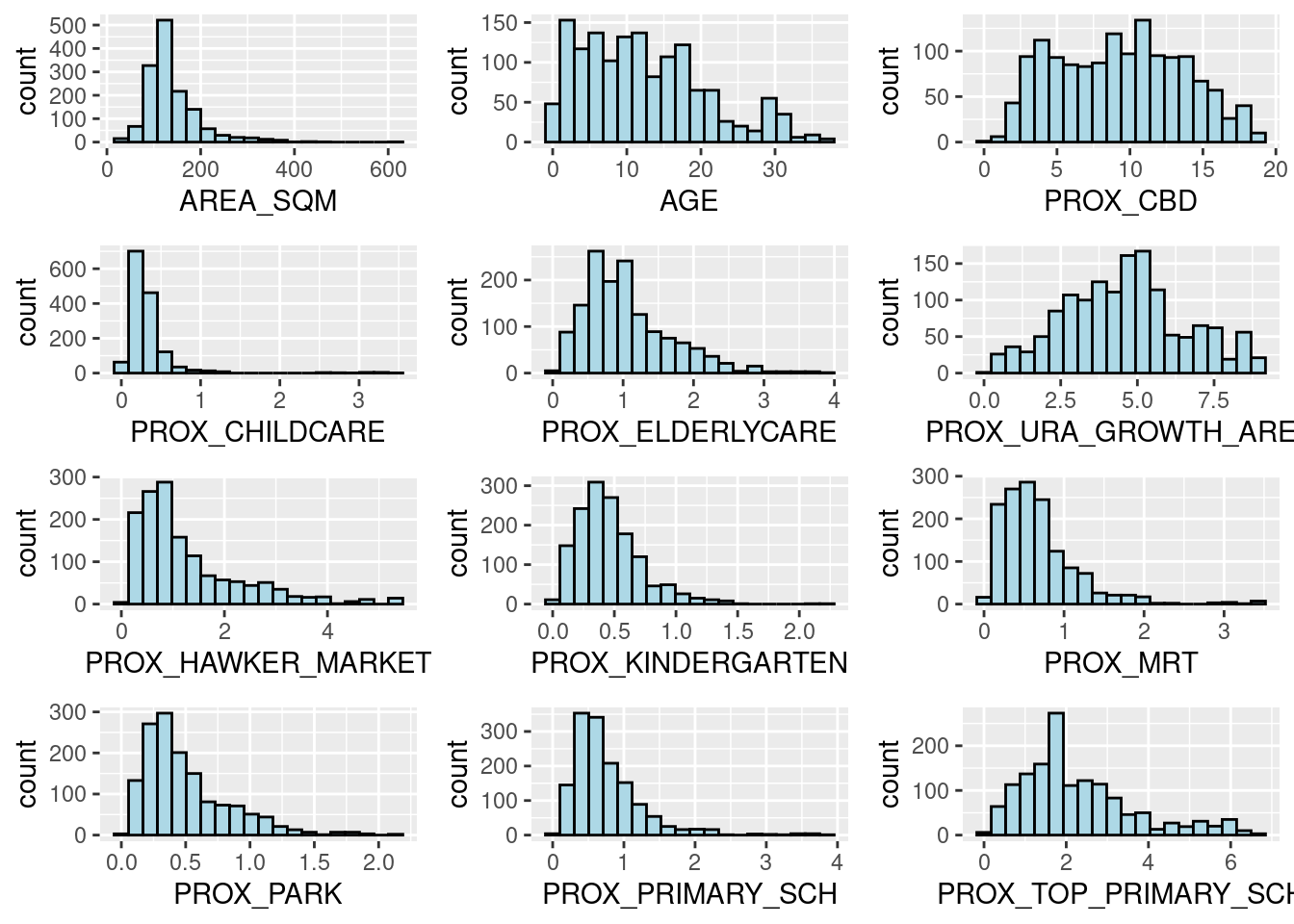
Statistical point map
We can visualise the distribution of condominium resale prices in Singapore using tmap.
tmap_mode("view")tmap mode set to interactive viewingtmap_options(check.and.fix = TRUE)
tm_shape(mpsz_svy21)+
tm_polygons() +
tm_shape(condo_resale.sf) +
tm_dots(col = "SELLING_PRICE",
alpha = 0.6,
style="quantile") +
tm_view(set.zoom.limits = c(11,14))Warning: The shape mpsz_svy21 is invalid (after reprojection). See
sf::st_is_validtmap_mode("plot")tmap mode set to plottingset.zoom.limits argument of tm_view sets the minimum and maximum zoom level to 11 and 14 respectively.
Hedonic pricing modelling
Hedonic pricing models (HPM) are methods used to estimate the value of a product or service by breaking it down into its individual features. These models assume that the price of something is based on its specific characteristics, and each feature adds to the overall value. This approach is especially useful for products like houses or cars, where the price is not just determined by the item itself but by its various qualities.
For example, when pricing a house, factors like location, size, number of bedrooms, and special features (like a pool or a garden) all influence its overall value. Hedonic pricing helps us figure out how much each of these features is worth in the total price.
Simple linear regression method
First, we will build a simple linear regression model by using SELLING_PRICE as the dependent variable and AREA_SQM as the independent variable.
The dependent variable is the outcome or the value that you are trying to explain or predict. In hedonic pricing models, this is usually the price of the product or service. For example, if you’re analyzing real estate prices, the price of the house (or condominium unit) would be the dependent variable. The dependent variable depends on the characteristics (or features) of the product.
The independent variables are the factors or characteristics that you believe influence the dependent variable. In hedonic pricing, these are the attributes of the product or service that are thought to contribute to its price.
condo.slr <- lm(formula=SELLING_PRICE ~ AREA_SQM, data = condo_resale.sf)You can use the summary() and anova() functions to get and print a summary or an analysis of variance (ANOVA) table from the results of the lm() function. There are also other helpful functions like coefficients, effects, fitted.values, and residuals that allow you to pull out specific details, such as the model’s coefficients, effects, predicted values, and residuals, from the results returned by lm().
summary(condo.slr)
Call:
lm(formula = SELLING_PRICE ~ AREA_SQM, data = condo_resale.sf)
Residuals:
Min 1Q Median 3Q Max
-3695815 -391764 -87517 258900 13503875
Coefficients:
Estimate Std. Error t value Pr(>|t|)
(Intercept) -258121.1 63517.2 -4.064 5.09e-05 ***
AREA_SQM 14719.0 428.1 34.381 < 2e-16 ***
---
Signif. codes: 0 '***' 0.001 '**' 0.01 '*' 0.05 '.' 0.1 ' ' 1
Residual standard error: 942700 on 1434 degrees of freedom
Multiple R-squared: 0.4518, Adjusted R-squared: 0.4515
F-statistic: 1182 on 1 and 1434 DF, p-value: < 2.2e-16The output report reveals that the SELLING_PRICE can be explained by using the formula:
SELLING_PRICE=−258,121.1+14,719×AREA_SQMSince the p-value is much smaller than 0.0001, we reject the null hypothesis that the mean is a good estimator of SELLING_PRICE, allowing us to conclude that the simple linear regression model provides a better estimate.
The “Coefficients” section of the report shows that the p-values for both the Intercept and AREA_SQM estimates are smaller than 0.001. Therefore, we reject the null hypothesis that (B0) and (B1) are equal to 0. As a result, we can conclude that (B0) (the intercept) and (B1) (the coefficient for AREA_SQM) are reliable parameter estimates for the model.
To visualize the best fit line on a scatterplot, we can use lm as a method function within ggplot’s geometry, as demonstrated in the code snippet below.
ggplot(data=condo_resale.sf,
aes(x=`AREA_SQM`, y=`SELLING_PRICE`)) +
geom_point() +
geom_smooth(method = lm)`geom_smooth()` using formula = 'y ~ x'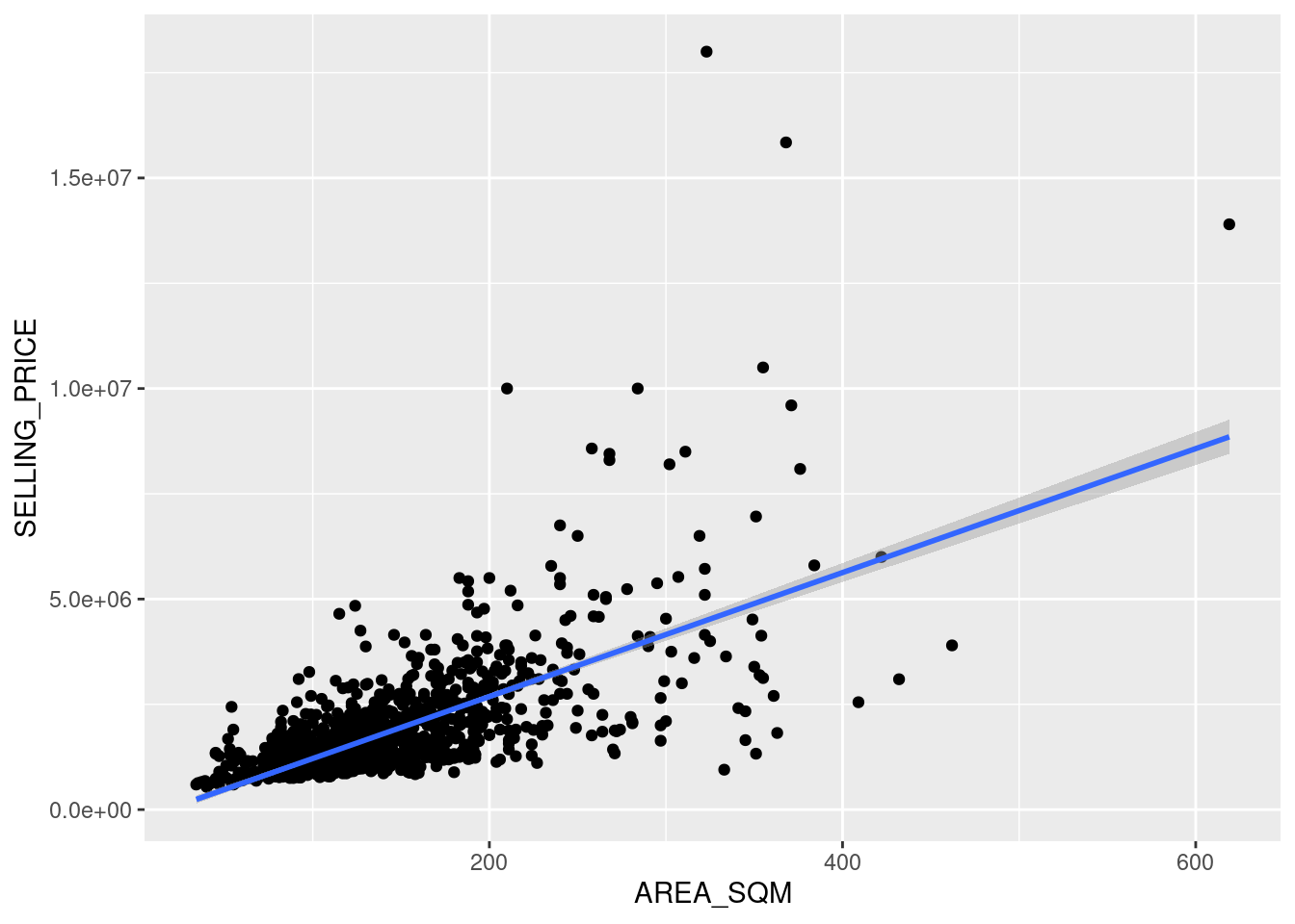
Figure above reveals that there are a few statistical outliers with relatively high selling prices.
Multiple linear regression model
Before building a multiple regression model, it’s important to make sure that the independent variables are not highly correlated with each other. If highly correlated variables are mistakenly included in the model, it can reduce the model’s accuracy, a problem known as multicollinearity in statistics.
A correlation matrix is often used to visualize the relationships between independent variables. In addition to the pairs function in R, there are many packages that can display a correlation matrix. In this section, we will use the corrplot package.
The code snippet below generates a scatterplot matrix to show the relationships between the independent variables in the condo_resale data frame.
corrplot(cor(condo_resale[, 5:23]), diag = FALSE, order = "AOE",
tl.pos = "td", tl.cex = 0.5, method = "number", type = "upper")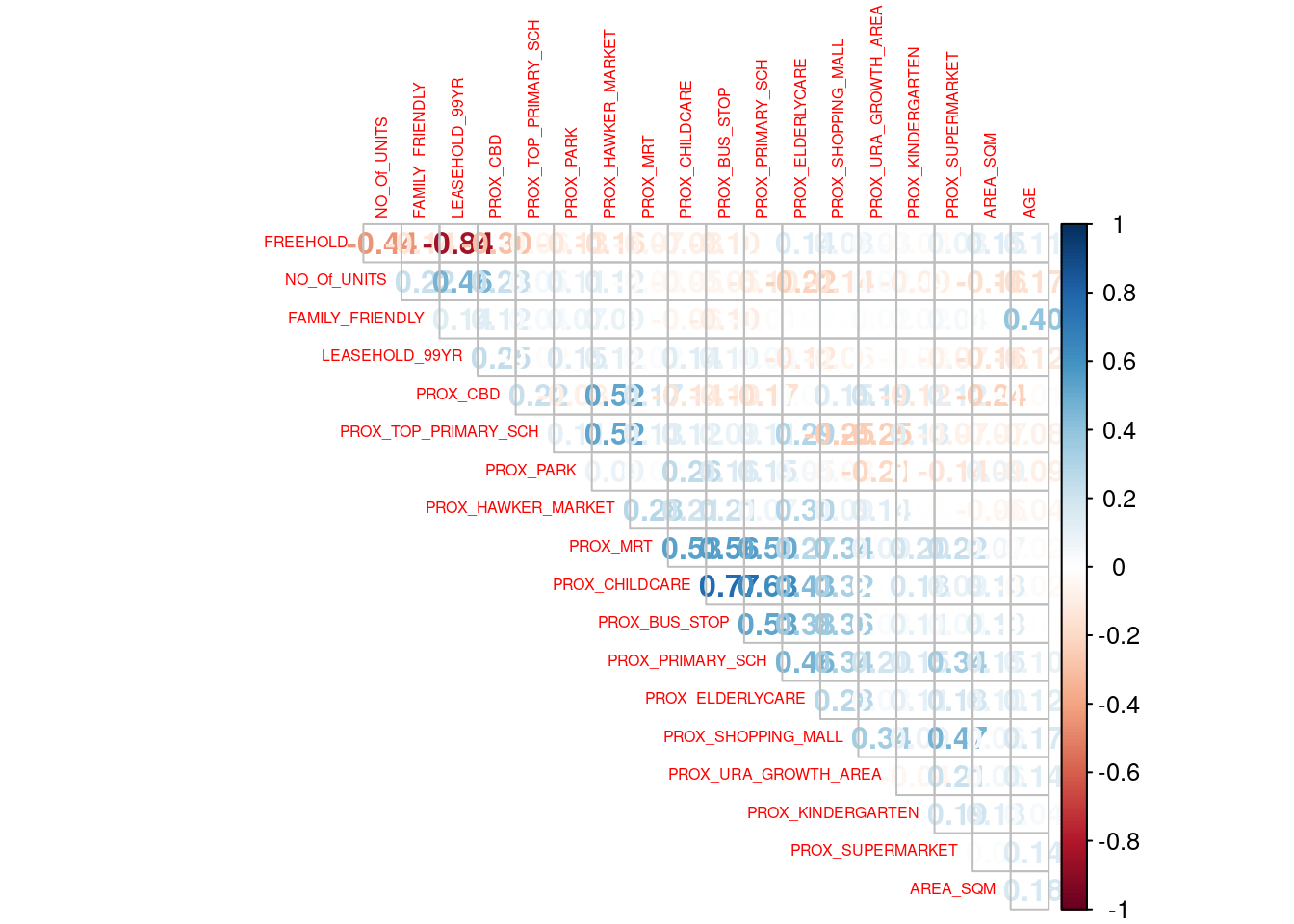
Reordering a matrix is crucial for uncovering hidden structures and patterns within the data. The corrplot package provides four reordering methods (via the order parameter): “AOE”, “FPC”, “hclust”, and “alphabet”. In the previous code chunk, the “AOE” method was used, which arranges variables using the angular order of eigenvectors, as recommended by Michael Friendly.
From the scatterplot matrix, it is evident that Freehold is highly correlated with LEASE_99YEAR. To avoid multicollinearity, it is better to include only one of these variables in the model. Therefore, LEASE_99YEAR is excluded from the subsequent model building.
Building a hedonic pricing model using multiple linear regression method
The code chunk below using lm to calibrate the multiple linear regression model.
condo.mlr <- lm(formula = SELLING_PRICE ~ AREA_SQM + AGE +
PROX_CBD + PROX_CHILDCARE + PROX_ELDERLYCARE +
PROX_URA_GROWTH_AREA + PROX_HAWKER_MARKET + PROX_KINDERGARTEN +
PROX_MRT + PROX_PARK + PROX_PRIMARY_SCH +
PROX_TOP_PRIMARY_SCH + PROX_SHOPPING_MALL + PROX_SUPERMARKET +
PROX_BUS_STOP + NO_Of_UNITS + FAMILY_FRIENDLY + FREEHOLD,
data=condo_resale.sf)
summary(condo.mlr)
Call:
lm(formula = SELLING_PRICE ~ AREA_SQM + AGE + PROX_CBD + PROX_CHILDCARE +
PROX_ELDERLYCARE + PROX_URA_GROWTH_AREA + PROX_HAWKER_MARKET +
PROX_KINDERGARTEN + PROX_MRT + PROX_PARK + PROX_PRIMARY_SCH +
PROX_TOP_PRIMARY_SCH + PROX_SHOPPING_MALL + PROX_SUPERMARKET +
PROX_BUS_STOP + NO_Of_UNITS + FAMILY_FRIENDLY + FREEHOLD,
data = condo_resale.sf)
Residuals:
Min 1Q Median 3Q Max
-3475964 -293923 -23069 241043 12260381
Coefficients:
Estimate Std. Error t value Pr(>|t|)
(Intercept) 481728.40 121441.01 3.967 7.65e-05 ***
AREA_SQM 12708.32 369.59 34.385 < 2e-16 ***
AGE -24440.82 2763.16 -8.845 < 2e-16 ***
PROX_CBD -78669.78 6768.97 -11.622 < 2e-16 ***
PROX_CHILDCARE -351617.91 109467.25 -3.212 0.00135 **
PROX_ELDERLYCARE 171029.42 42110.51 4.061 5.14e-05 ***
PROX_URA_GROWTH_AREA 38474.53 12523.57 3.072 0.00217 **
PROX_HAWKER_MARKET 23746.10 29299.76 0.810 0.41782
PROX_KINDERGARTEN 147468.99 82668.87 1.784 0.07466 .
PROX_MRT -314599.68 57947.44 -5.429 6.66e-08 ***
PROX_PARK 563280.50 66551.68 8.464 < 2e-16 ***
PROX_PRIMARY_SCH 180186.08 65237.95 2.762 0.00582 **
PROX_TOP_PRIMARY_SCH 2280.04 20410.43 0.112 0.91107
PROX_SHOPPING_MALL -206604.06 42840.60 -4.823 1.57e-06 ***
PROX_SUPERMARKET -44991.80 77082.64 -0.584 0.55953
PROX_BUS_STOP 683121.35 138353.28 4.938 8.85e-07 ***
NO_Of_UNITS -231.18 89.03 -2.597 0.00951 **
FAMILY_FRIENDLY 140340.77 47020.55 2.985 0.00289 **
FREEHOLD 359913.01 49220.22 7.312 4.38e-13 ***
---
Signif. codes: 0 '***' 0.001 '**' 0.01 '*' 0.05 '.' 0.1 ' ' 1
Residual standard error: 755800 on 1417 degrees of freedom
Multiple R-squared: 0.6518, Adjusted R-squared: 0.6474
F-statistic: 147.4 on 18 and 1417 DF, p-value: < 2.2e-16Based on the report above, it is clear that not all the independent variables are statistically significant. We will revise the model by removing those variables that are not statistically significant.
With this adjustment, we are now ready to fit the revised model using the code snippet below.
condo.mlr1 <- lm(formula = SELLING_PRICE ~ AREA_SQM + AGE +
PROX_CBD + PROX_CHILDCARE + PROX_ELDERLYCARE +
PROX_URA_GROWTH_AREA + PROX_MRT + PROX_PARK +
PROX_PRIMARY_SCH + PROX_SHOPPING_MALL + PROX_BUS_STOP +
NO_Of_UNITS + FAMILY_FRIENDLY + FREEHOLD,
data=condo_resale.sf)
ols_regress(condo.mlr1) Model Summary
-----------------------------------------------------------------------------
R 0.807 RMSE 751998.679
R-Squared 0.651 MSE 571471422208.591
Adj. R-Squared 0.647 Coef. Var 43.168
Pred R-Squared 0.638 AIC 42966.758
MAE 414819.628 SBC 43051.072
-----------------------------------------------------------------------------
RMSE: Root Mean Square Error
MSE: Mean Square Error
MAE: Mean Absolute Error
AIC: Akaike Information Criteria
SBC: Schwarz Bayesian Criteria
ANOVA
--------------------------------------------------------------------------------
Sum of
Squares DF Mean Square F Sig.
--------------------------------------------------------------------------------
Regression 1.512586e+15 14 1.080418e+14 189.059 0.0000
Residual 8.120609e+14 1421 571471422208.591
Total 2.324647e+15 1435
--------------------------------------------------------------------------------
Parameter Estimates
-----------------------------------------------------------------------------------------------------------------
model Beta Std. Error Std. Beta t Sig lower upper
-----------------------------------------------------------------------------------------------------------------
(Intercept) 527633.222 108183.223 4.877 0.000 315417.244 739849.200
AREA_SQM 12777.523 367.479 0.584 34.771 0.000 12056.663 13498.382
AGE -24687.739 2754.845 -0.167 -8.962 0.000 -30091.739 -19283.740
PROX_CBD -77131.323 5763.125 -0.263 -13.384 0.000 -88436.469 -65826.176
PROX_CHILDCARE -318472.751 107959.512 -0.084 -2.950 0.003 -530249.889 -106695.613
PROX_ELDERLYCARE 185575.623 39901.864 0.090 4.651 0.000 107302.737 263848.510
PROX_URA_GROWTH_AREA 39163.254 11754.829 0.060 3.332 0.001 16104.571 62221.936
PROX_MRT -294745.107 56916.367 -0.112 -5.179 0.000 -406394.234 -183095.980
PROX_PARK 570504.807 65507.029 0.150 8.709 0.000 442003.938 699005.677
PROX_PRIMARY_SCH 159856.136 60234.599 0.062 2.654 0.008 41697.849 278014.424
PROX_SHOPPING_MALL -220947.251 36561.832 -0.115 -6.043 0.000 -292668.213 -149226.288
PROX_BUS_STOP 682482.221 134513.243 0.134 5.074 0.000 418616.359 946348.082
NO_Of_UNITS -245.480 87.947 -0.053 -2.791 0.005 -418.000 -72.961
FAMILY_FRIENDLY 146307.576 46893.021 0.057 3.120 0.002 54320.593 238294.560
FREEHOLD 350599.812 48506.485 0.136 7.228 0.000 255447.802 445751.821
-----------------------------------------------------------------------------------------------------------------The gtsummary package offers an elegant and versatile approach for creating publication-ready summary tables in R.
In the code snippet below, tbl_regression is used to generate a neatly formatted regression report.
tbl_regression(condo.mlr1, intercept = TRUE)| Characteristic | Beta | 95% CI1 | p-value |
|---|---|---|---|
| (Intercept) | 527,633 | 315,417, 739,849 | <0.001 |
| AREA_SQM | 12,778 | 12,057, 13,498 | <0.001 |
| AGE | -24,688 | -30,092, -19,284 | <0.001 |
| PROX_CBD | -77,131 | -88,436, -65,826 | <0.001 |
| PROX_CHILDCARE | -318,473 | -530,250, -106,696 | 0.003 |
| PROX_ELDERLYCARE | 185,576 | 107,303, 263,849 | <0.001 |
| PROX_URA_GROWTH_AREA | 39,163 | 16,105, 62,222 | <0.001 |
| PROX_MRT | -294,745 | -406,394, -183,096 | <0.001 |
| PROX_PARK | 570,505 | 442,004, 699,006 | <0.001 |
| PROX_PRIMARY_SCH | 159,856 | 41,698, 278,014 | 0.008 |
| PROX_SHOPPING_MALL | -220,947 | -292,668, -149,226 | <0.001 |
| PROX_BUS_STOP | 682,482 | 418,616, 946,348 | <0.001 |
| NO_Of_UNITS | -245 | -418, -73 | 0.005 |
| FAMILY_FRIENDLY | 146,308 | 54,321, 238,295 | 0.002 |
| FREEHOLD | 350,600 | 255,448, 445,752 | <0.001 |
| 1 CI = Confidence Interval | |||
Using the gtsummary package, model statistics can be incorporated into the report either by appending them directly to the table with add_glance_table or by adding them as a source note with add_glance_source_note, as demonstrated in the code snippet below.
tbl_regression(condo.mlr1,
intercept = TRUE) %>%
add_glance_source_note(
label = list(sigma ~ "\U03C3"),
include = c(r.squared, adj.r.squared,
AIC, statistic,
p.value, sigma))| Characteristic | Beta | 95% CI1 | p-value |
|---|---|---|---|
| (Intercept) | 527,633 | 315,417, 739,849 | <0.001 |
| AREA_SQM | 12,778 | 12,057, 13,498 | <0.001 |
| AGE | -24,688 | -30,092, -19,284 | <0.001 |
| PROX_CBD | -77,131 | -88,436, -65,826 | <0.001 |
| PROX_CHILDCARE | -318,473 | -530,250, -106,696 | 0.003 |
| PROX_ELDERLYCARE | 185,576 | 107,303, 263,849 | <0.001 |
| PROX_URA_GROWTH_AREA | 39,163 | 16,105, 62,222 | <0.001 |
| PROX_MRT | -294,745 | -406,394, -183,096 | <0.001 |
| PROX_PARK | 570,505 | 442,004, 699,006 | <0.001 |
| PROX_PRIMARY_SCH | 159,856 | 41,698, 278,014 | 0.008 |
| PROX_SHOPPING_MALL | -220,947 | -292,668, -149,226 | <0.001 |
| PROX_BUS_STOP | 682,482 | 418,616, 946,348 | <0.001 |
| NO_Of_UNITS | -245 | -418, -73 | 0.005 |
| FAMILY_FRIENDLY | 146,308 | 54,321, 238,295 | 0.002 |
| FREEHOLD | 350,600 | 255,448, 445,752 | <0.001 |
| R² = 0.651; Adjusted R² = 0.647; AIC = 42,967; Statistic = 189; p-value = <0.001; σ = 755,957 | |||
| 1 CI = Confidence Interval | |||
Checking for multicolinearity
In this section, we introduce an excellent R package designed specifically for performing OLS regression, called olsrr. This package offers a variety of helpful tools for building improved multiple linear regression models, including:
- Comprehensive regression output
- Residual diagnostics
- Measures of influence
- Heteroskedasticity tests
- Collinearity diagnostics
- Model fit assessment
- Variable contribution evaluation
- Variable selection procedures
In the code snippet below, the ols_vif_tol function from the olsrr package is used to check for signs of multicollinearity.
ols_vif_tol(condo.mlr1) Variables Tolerance VIF
1 AREA_SQM 0.8728554 1.145665
2 AGE 0.7071275 1.414172
3 PROX_CBD 0.6356147 1.573280
4 PROX_CHILDCARE 0.3066019 3.261559
5 PROX_ELDERLYCARE 0.6598479 1.515501
6 PROX_URA_GROWTH_AREA 0.7510311 1.331503
7 PROX_MRT 0.5236090 1.909822
8 PROX_PARK 0.8279261 1.207837
9 PROX_PRIMARY_SCH 0.4524628 2.210126
10 PROX_SHOPPING_MALL 0.6738795 1.483945
11 PROX_BUS_STOP 0.3514118 2.845664
12 NO_Of_UNITS 0.6901036 1.449058
13 FAMILY_FRIENDLY 0.7244157 1.380423
14 FREEHOLD 0.6931163 1.442759Since the VIF of the independent variables are less than 10. We can safely conclude that there are no sign of multicollinearity among the independent variables.
Test for non-linearity
In multiple linear regression, it’s essential to test the assumption of linearity and additivity in the relationship between the dependent and independent variables.
In the code snippet below, the ols_plot_resid_fit function from the olsrr package is used to assess the linearity assumption.
ols_plot_resid_fit(condo.mlr1)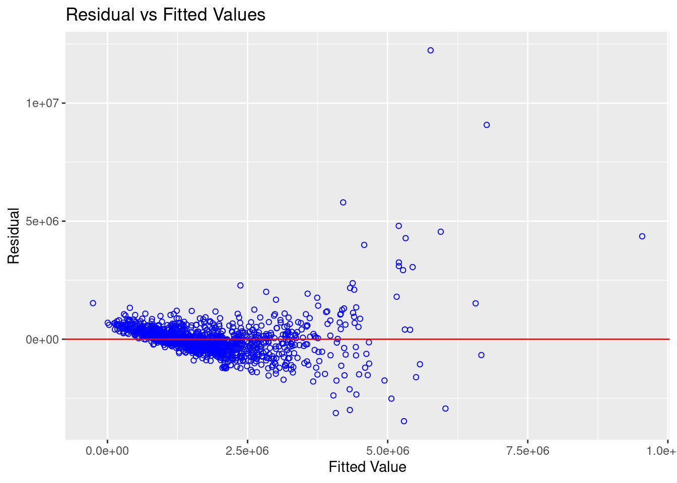
The figure above reveals that most of the data poitns are scattered around the 0 line, hence we can safely conclude that the relationships between the dependent variable and independent variables are linear.
Test for normality assumption
Finally, the code snippet below uses the ols_plot_resid_hist function from the olsrr package to test the normality assumption.
ols_plot_resid_hist(condo.mlr1)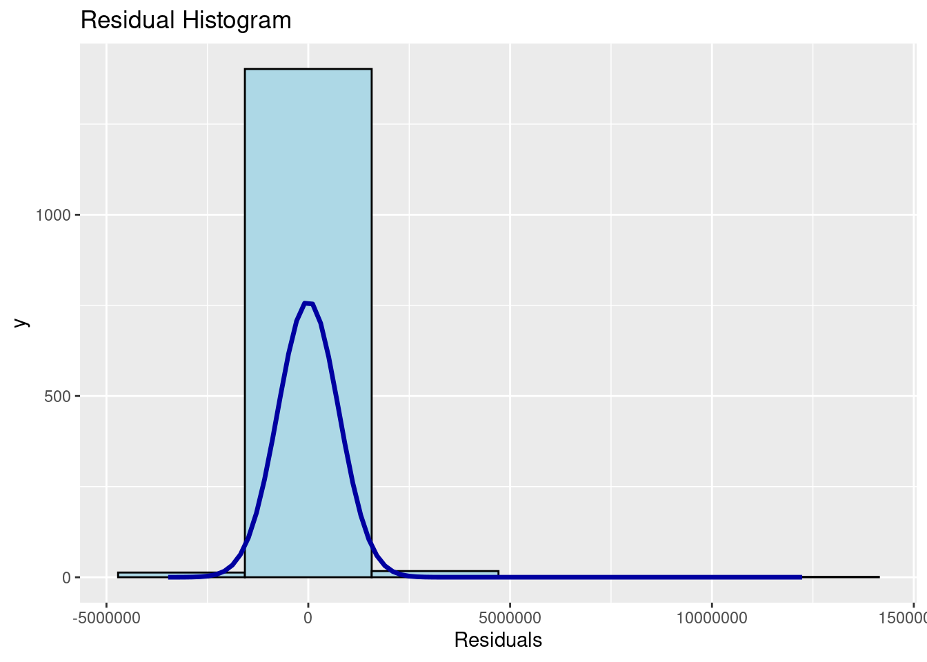
The figure shows that the residuals of the multiple linear regression model (i.e., condo.mlr1) resemble a normal distribution.
If you prefer formal statistical testing, you can use the ols_test_normality function from the olsrr package, as demonstrated in the code snippet below.
ols_test_normality(condo.mlr1)Warning in ks.test.default(y, "pnorm", mean(y), sd(y)): ties should not be
present for the one-sample Kolmogorov-Smirnov test-----------------------------------------------
Test Statistic pvalue
-----------------------------------------------
Shapiro-Wilk 0.6856 0.0000
Kolmogorov-Smirnov 0.1366 0.0000
Cramer-von Mises 121.0768 0.0000
Anderson-Darling 67.9551 0.0000
-----------------------------------------------The summary table above reveals that the p-values of the four tests are way smaller than the alpha value of 0.05. Hence we will reject the null hypothesis and infer that there is statistical evidence that the residual are not normally distributed.
Testing for spatial auto-correlation
The hedonic model we are building incorporates geographically referenced attributes, so it is important to visualize the residuals of the hedonic pricing model.
To perform a spatial autocorrelation test, we first need to convert condo_resale.sf from an sf data frame into a SpatialPointsDataFrame.
As a first step, we will export the residuals of the hedonic pricing model and save them as a data frame.
mlr.output <- as.data.frame(condo.mlr1$residuals)Next, we will merge the newly created data frame with the condo_resale.sf object.
condo_resale.res.sf <- cbind(condo_resale.sf,
condo.mlr1$residuals) %>%
rename(`MLR_RES` = `condo.mlr1.residuals`)Next, we will convert condo_resale.res.sf from simple feature object into a SpatialPointsDataFrame because spdep package can only process sp conformed spatial data objects.
The code chunk below will be used to perform the data conversion process.
condo_resale.sp <- as_Spatial(condo_resale.res.sf)
condo_resale.spclass : SpatialPointsDataFrame
features : 1436
extent : 14940.85, 43352.45, 24765.67, 48382.81 (xmin, xmax, ymin, ymax)
crs : +proj=tmerc +lat_0=1.36666666666667 +lon_0=103.833333333333 +k=1 +x_0=28001.642 +y_0=38744.572 +ellps=WGS84 +towgs84=0,0,0,0,0,0,0 +units=m +no_defs
variables : 23
names : POSTCODE, SELLING_PRICE, AREA_SQM, AGE, PROX_CBD, PROX_CHILDCARE, PROX_ELDERLYCARE, PROX_URA_GROWTH_AREA, PROX_HAWKER_MARKET, PROX_KINDERGARTEN, PROX_MRT, PROX_PARK, PROX_PRIMARY_SCH, PROX_TOP_PRIMARY_SCH, PROX_SHOPPING_MALL, ...
min values : 18965, 540000, 34, 0, 0.386916393, 0.004927023, 0.054508623, 0.214539508, 0.051817113, 0.004927023, 0.052779424, 0.029064164, 0.077106132, 0.077106132, 0, ...
max values : 828833, 1.8e+07, 619, 37, 19.18042832, 3.46572633, 3.949157205, 9.15540001, 5.374348075, 2.229045366, 3.48037319, 2.16104919, 3.928989144, 6.748192062, 3.477433767, ... Next, we will use tmap package to display the distribution of the residuals on an interactive map.
tmap_mode("view")tmap mode set to interactive viewingtm_shape(mpsz_svy21)+
tmap_options(check.and.fix = TRUE) +
tm_polygons(alpha = 0.4) +
tm_shape(condo_resale.res.sf) +
tm_dots(col = "MLR_RES",
alpha = 0.6,
style="quantile") +
tm_view(set.zoom.limits = c(11,14))Warning: The shape mpsz_svy21 is invalid (after reprojection). See
sf::st_is_validVariable(s) "MLR_RES" contains positive and negative values, so midpoint is set to 0. Set midpoint = NA to show the full spectrum of the color palette.tmap_mode("plot")tmap mode set to plottingThe figure above indicates signs of spatial autocorrelation.
To confirm this observation, we will perform Moran’s I test.
First, we will calculate the distance-based weight matrix using the dnearneigh() function from the spdep package.
nb <- dnearneigh(coordinates(condo_resale.sp), 0, 1500, longlat = FALSE)Warning in dnearneigh(coordinates(condo_resale.sp), 0, 1500, longlat = FALSE):
neighbour object has 10 sub-graphssummary(nb)Neighbour list object:
Number of regions: 1436
Number of nonzero links: 66266
Percentage nonzero weights: 3.213526
Average number of links: 46.14624
10 disjoint connected subgraphs
Link number distribution:
1 3 5 7 9 10 11 12 13 14 15 16 17 18 19 20 21 22 23 24
3 3 9 4 3 15 10 19 17 45 19 5 14 29 19 6 35 45 18 47
25 26 27 28 29 30 31 32 33 34 35 36 37 38 39 40 41 42 43 44
16 43 22 26 21 11 9 23 22 13 16 25 21 37 16 18 8 21 4 12
45 46 47 48 49 50 51 52 53 54 55 56 57 58 59 60 61 62 63 64
8 36 18 14 14 43 11 12 8 13 12 13 4 5 6 12 11 20 29 33
65 66 67 68 69 70 71 72 73 74 75 76 77 78 79 80 81 82 83 84
15 20 10 14 15 15 11 16 12 10 8 19 12 14 9 8 4 13 11 6
85 86 87 88 89 90 91 92 93 94 95 96 97 98 99 100 101 102 103 104
4 9 4 4 4 6 2 16 9 4 5 9 3 9 4 2 1 2 1 1
105 106 107 108 109 110 112 116 125
1 5 9 2 1 3 1 1 1
3 least connected regions:
193 194 277 with 1 link
1 most connected region:
285 with 125 linksNext, the nb2listw function from the spdep package will be used to convert the neighbor list (i.e., nb) into spatial weights.
nb_lw <- nb2listw(nb, style = 'W')
summary(nb_lw)Characteristics of weights list object:
Neighbour list object:
Number of regions: 1436
Number of nonzero links: 66266
Percentage nonzero weights: 3.213526
Average number of links: 46.14624
10 disjoint connected subgraphs
Link number distribution:
1 3 5 7 9 10 11 12 13 14 15 16 17 18 19 20 21 22 23 24
3 3 9 4 3 15 10 19 17 45 19 5 14 29 19 6 35 45 18 47
25 26 27 28 29 30 31 32 33 34 35 36 37 38 39 40 41 42 43 44
16 43 22 26 21 11 9 23 22 13 16 25 21 37 16 18 8 21 4 12
45 46 47 48 49 50 51 52 53 54 55 56 57 58 59 60 61 62 63 64
8 36 18 14 14 43 11 12 8 13 12 13 4 5 6 12 11 20 29 33
65 66 67 68 69 70 71 72 73 74 75 76 77 78 79 80 81 82 83 84
15 20 10 14 15 15 11 16 12 10 8 19 12 14 9 8 4 13 11 6
85 86 87 88 89 90 91 92 93 94 95 96 97 98 99 100 101 102 103 104
4 9 4 4 4 6 2 16 9 4 5 9 3 9 4 2 1 2 1 1
105 106 107 108 109 110 112 116 125
1 5 9 2 1 3 1 1 1
3 least connected regions:
193 194 277 with 1 link
1 most connected region:
285 with 125 links
Weights style: W
Weights constants summary:
n nn S0 S1 S2
W 1436 2062096 1436 94.81916 5798.341Next, the lm.morantest function from the spdep package will be used to conduct Moran’s I test for residual spatial autocorrelation.
lm.morantest(condo.mlr1, nb_lw)
Global Moran I for regression residuals
data:
model: lm(formula = SELLING_PRICE ~ AREA_SQM + AGE + PROX_CBD +
PROX_CHILDCARE + PROX_ELDERLYCARE + PROX_URA_GROWTH_AREA + PROX_MRT +
PROX_PARK + PROX_PRIMARY_SCH + PROX_SHOPPING_MALL + PROX_BUS_STOP +
NO_Of_UNITS + FAMILY_FRIENDLY + FREEHOLD, data = condo_resale.sf)
weights: nb_lw
Moran I statistic standard deviate = 24.366, p-value < 2.2e-16
alternative hypothesis: greater
sample estimates:
Observed Moran I Expectation Variance
1.438876e-01 -5.487594e-03 3.758259e-05 The Global Moran’s I test for residual spatial autocorrelation shows that it’s p-value is less than 0.00000000000000022 which is less than the alpha value of 0.05. Hence, we will reject the null hypothesis that the residuals are randomly distributed.
Since the Observed Global Moran I = 0.1424418 which is greater than 0, we can infer than the residuals resemble cluster distribution.